computed tomography (CT) images of the lumbar spine. The resulting mean symmetric absolute surface distance of  mm and Dice coefficient of
  %, computed from the final vertebra detection results against corresponding reference vertebra segmentations, indicate that the proposed framework can successfully detected vertebrae in CT images of the lumbar spine.
1 Introduction
Detection and segmentation of an object of interest can always be represented as a specific optimization problem. As optimization problems are usually non-deterministic polynomial-time hard (NP-hard) or non-analytically defined, they can be solved by brute force algorithms that are computationally demanding or by heuristic approaches that may not find the globally optimal solution. Moreover, if the optimization problem is ill-posed, there is no guarantee that the optimal detection or segmentation result is associated with the global optimum of the problem. Such lack of correspondence is observed in the case of vertebra detection in medical images of the spine, where neighboring vertebrae are of similar appearance and shape, which often causes mis-detections. We can therefore conclude that there is a need for an optimizer that will consider not only the global optimum but also local optima of the problem that represent candidate locations for each vertebra, and that can be further used for accurate and robust spine and vertebra detection. As standard optimization techniques, such as the Powell’s optimizer [1] or covariance matrix adaptation evolution strategy (CMA-ES) [2], detect only a single local optimum, we propose to use interpolation theory to overcome the above mentioned limitations and ensure the detection of all local optima. Interpolation theory estimates the behavior of smooth functions according to a small set of points, for which the behavior is known. In the case of object detection, interpolation theory can predict the position of the object of interest by computing a specified detector response for a sparse set of points, i.e. possible transformations of the object of interest. In this paper, we describe a novel framework for automated spine and vertebra detection in three-dimensional (3D) computed tomography (CT) images of the lumbar spine, where we first apply interpolation-based optimization to detect the location of the whole lumbar spine in the 3D image, and then detect the location of individual lumbar vertebrae within the spinal column.
2 Methodology
Detection of the object of interest (e.g. spine, vertebra) in an unknown 3D image  can be, in general, performed by optimizing an objective function
  , which maps the model of the object of interest, represented by a set
  of
of  parameters describing its geometrical properties (e.g. position, rotation, scaling etc.), to image
  in
in  -dimensional parameter space. The most straightforward but computationally demanding approach for optimizing
  is to apply brute force to compute its response for all
  , where
  is a bounded domain in the parameter space. Alternative approaches [1, 2] often compute function responses in a neighborhood of an initial set
  , predict the optimal
  and iteratively move towards
  . Although such optimization is computationally not demanding and may, especially if
  is relatively close to
  , lead to the globally optimal solution, it may still converge to local optima. Therefore, there is a need to observe the whole
  and, at the same time, minimize actual computations of
  . To overcome these problems, we propose a novel optimization scheme that is based on interpolation theory [3]. The proposed optimization scheme does not depend on initialization and observes the whole
  , and we apply it for spine and vertebra detection in 3D spine images. Depending on the objective function
  , the scheme searches for optima in the form of either minima or maxima, however, we will refer to them as maxima in the following text.
can be, in general, performed by optimizing an objective function , which maps the model of the object of interest, represented by a set of parameters describing its geometrical properties (e.g. position, rotation, scaling etc.), to image in -dimensional parameter space. The most straightforward but computationally demanding approach for optimizing is to apply brute force to compute its response for all , where is a bounded domain in the parameter space. Alternative approaches [1, 2] often compute function responses in a neighborhood of an initial set , predict the optimal and iteratively move towards . Although such optimization is computationally not demanding and may, especially if is relatively close to , lead to the globally optimal solution, it may still converge to local optima. Therefore, there is a need to observe the whole and, at the same time, minimize actual computations of . To overcome these problems, we propose a novel optimization scheme that is based on interpolation theory [3]. The proposed optimization scheme does not depend on initialization and observes the whole , and we apply it for spine and vertebra detection in 3D spine images. Depending on the objective function , the scheme searches for optima in the form of either minima or maxima, however, we will refer to them as maxima in the following text.Fig. 1
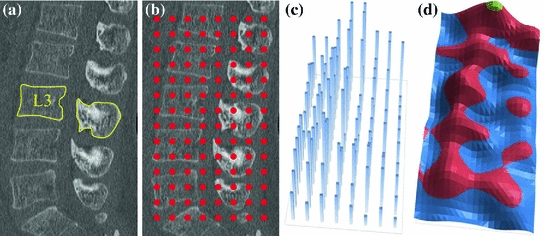
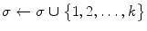
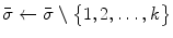
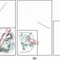
An illustration of the L3 vertebra detection. a Reference segmentation binary mask, overlayed onto a selected sagittal cross-section of the CT image. b The interpolation grid. c The objective function  is computed only for nodes forming the interpolation grid. d The local maxima of the interpolation function
  indicate candidate locations of the observed vertebra. In this case, the global maximum (in green) does not correspond to the location of L3 (Color figure online)
is computed only for nodes forming the interpolation grid. d The local maxima of the interpolation function indicate candidate locations of the observed vertebra. In this case, the global maximum (in green) does not correspond to the location of L3 (Color figure online)2.1 Interpolation Theory
By assuming that the objective function  is smooth and its values are similar for similar sets
  of parameters,
  can be approximated by function
  if the response of
  is known for a limited set of nodes
  (Fig. 1). If nodes in
  are selected properly, the difference between
  and its approximation
  , i.e. the interpolation error, is relatively small, and the maximum of
  corresponds to the maximum of
  at the same point
  . The main concept of interpolation theory [3] is to select the interpolation function, in our case
  , from a given class of functions so that its response passes through the nodes in
  , which form the interpolation grid over the observed domain
  . However, interpolation of high-dimensional functions is computationally challenging, as the number of nodes grows exponentially with the increasing number of dimensions
  . To reduce the computational complexity, various strategies can be applied [4, 5], but in our case we take into account the properties of spine detection. The standard spine image acquisition procedure restricts the orientation of the imaged subject, and therefore the relative inclination of the spinal column in the image is more constant than its position, and similarly the orientation of a vertebra is restricted by the position of neighboring vertebrae. It can be concluded that dimensions related to object translation have to be associated with a larger number of interpolation nodes than dimensions related to object rotations. To optimize the objective function
  , defined on domain
  of
of  dimensions, we therefore propose the following algorithm:
is smooth and its values are similar for similar sets of parameters, can be approximated by function if the response of is known for a limited set of nodes (Fig. 1). If nodes in are selected properly, the difference between and its approximation , i.e. the interpolation error, is relatively small, and the maximum of corresponds to the maximum of at the same point . The main concept of interpolation theory [3] is to select the interpolation function, in our case , from a given class of functions so that its response passes through the nodes in , which form the interpolation grid over the observed domain . However, interpolation of high-dimensional functions is computationally challenging, as the number of nodes grows exponentially with the increasing number of dimensions . To reduce the computational complexity, various strategies can be applied [4, 5], but in our case we take into account the properties of spine detection. The standard spine image acquisition procedure restricts the orientation of the imaged subject, and therefore the relative inclination of the spinal column in the image is more constant than its position, and similarly the orientation of a vertebra is restricted by the position of neighboring vertebrae. It can be concluded that dimensions related to object translation have to be associated with a larger number of interpolation nodes than dimensions related to object rotations. To optimize the objective function , defined on domain of dimensions, we therefore propose the following algorithm:1.
Initialize set  of optimized dimensions as
  , and set
  of the remaining dimensions as
 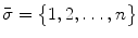 .
.
of optimized dimensions as , and set of the remaining dimensions as .2.
Interpolate  with
with  against the first
  dimensions.
with against the first dimensions.3.
Find  local maxima of
  , then insert the observed dimensions into
  ;
;  , and remove them from
  ;
;  .
.
local maxima of , then insert the observed dimensions into ; , and remove them from ; .4.
For each local maximum among  , perform the following steps:
, perform the following steps:4a.
If  , take the next
  available dimensions and interpolate
  with
with  by considering dimensions from
  to be optimized.
, take the next available dimensions and interpolate with by considering dimensions from to be optimized.4b.
Find the global maximum of  , insert the observed dimensions into
  and remove them from
  . Return to step 4a.
, insert the observed dimensions into and remove them from . Return to step 4a.5.
The resulting global maxima represent the locations of  local maxima of
  .
.
local maxima of .In the proposed algorithm, the optimization dimensions have to be ordered according to the decreasing number of corresponding interpolation nodes, while the number of dimensions  considered in each interpolation step may vary for different steps. Nevertheless, by taking into account only
  dimensions at once, the computational complexity of the high-dimensional optimization problem is reduced.
considered in each interpolation step may vary for different steps. Nevertheless, by taking into account only dimensions at once, the computational complexity of the high-dimensional optimization problem is reduced.2.2 Mean Shape Model of the Lumbar Spine
Let set  contain 3D images of the lumbar spine, where each image is assigned a series of binary masks representing reference segmentations of each individual lumbar vertebra from level L1 to L5. To extract a shape model of each vertebra from each image in
  , the marching cubes algorithm [6] is applied to each corresponding binary mask, resulting in a 3D face-vertex mesh consisting of vertices with triangle connectivity information. The dependency of the number of vertices in each mesh on the size of the image voxel and of the observed vertebra is removed by isotropic remeshing [7], and the coherent point drift algorithm [8] is used to recover the nonrigid transformation among sets of vertices and establish point wise correspondences among vertices of the same vertebral level. Finally, the generalized Procrustes alignment [9] is used to remove translation, rotation and scaling from corresponding meshes, yielding the mean shape model of each vertebra, represented by a 3D face-vertex mesh
  of
of  vertices and
  faces (i.e. triangles). The mean shape model of the whole lumbar spine, i.e. a chain of mean shape models of individual vertebrae, is further used for spine detection, while mean shape models of individual vertebrae are used for vertebra detection in an unknown 3D image
  .
.
contain 3D images of the lumbar spine, where each image is assigned a series of binary masks representing reference segmentations of each individual lumbar vertebra from level L1 to L5. To extract a shape model of each vertebra from each image in , the marching cubes algorithm [6] is applied to each corresponding binary mask, resulting in a 3D face-vertex mesh consisting of vertices with triangle connectivity information. The dependency of the number of vertices in each mesh on the size of the image voxel and of the observed vertebra is removed by isotropic remeshing [7], and the coherent point drift algorithm [8] is used to recover the nonrigid transformation among sets of vertices and establish point wise correspondences among vertices of the same vertebral level. Finally, the generalized Procrustes alignment [9] is used to remove translation, rotation and scaling from corresponding meshes, yielding the mean shape model of each vertebra, represented by a 3D face-vertex mesh of vertices and faces (i.e. triangles). The mean shape model of the whole lumbar spine, i.e. a chain of mean shape models of individual vertebrae, is further used for spine detection, while mean shape models of individual vertebrae are used for vertebra detection in an unknown 3D image .2.3 Spine Detection
Let the 3D mesh  represent the mean shape model of the lumbar spine (Sect. 2.2), i.e. a chain of meshes representing individual vertebrae from L1 to L5. The objective function
  that measures the agreement between mesh
  and image
  is defined as:
where  denotes the dot product,
  is the number of mesh vertices,
  is a mesh vertex,
  is the Haar-like gradient [10] of image
  at the location of vertex
  , and
, and  is the mesh normal at vertex
  . If mesh
  is correctly aligned with the spine in image
  , then mesh normals pointing outwards of the mesh are in maximal agreement with the Haar-like gradients pointing outwards of the spine, resulting in the maximum of the objective function
  . As Haar-like gradients are described as a difference between two neighboring cuboids instead of two neighboring voxels, they are not sensitive to local intensity fluctuations and therefore make spine detection more robust.
represent the mean shape model of the lumbar spine (Sect. 2.2), i.e. a chain of meshes representing individual vertebrae from L1 to L5. The objective function that measures the agreement between mesh and image is defined as:(1)
denotes the dot product, is the number of mesh vertices, is a mesh vertex, is the Haar-like gradient [10] of image at the location of vertex , and is the mesh normal at vertex . If mesh is correctly aligned with the spine in image , then mesh normals pointing outwards of the mesh are in maximal agreement with the Haar-like gradients pointing outwards of the spine, resulting in the maximum of the objective function . As Haar-like gradients are described as a difference between two neighboring cuboids instead of two neighboring voxels, they are not sensitive to local intensity fluctuations and therefore make spine detection more robust.Related posts:
 Models for Descriptive Patient-Specific Neuro-Anatomical Modeling: Towards a Digital Brainstem Atlas
 Supervised Segmentation and Meshing of 3D Intervertebral Discs of the Lumbar Spine for Discectomy Simulation
 Vertebral Segmentation Using Part-Based Decomposition and Conditional Shape Models
Stay updated, free articles. Join our Telegram channel

Full access? Get Clinical Tree


