Fig. 21.1
(Left–Middle–Right) The probabilities of throwing n eyes with 1, 2, and 5 dice, respectively, are shown
Similarly, rather than counting eyes on dice, one can also measure the distance traveled by a molecule given a diffusion time.
Free Diffusion
Einstein showed that the displacement of water molecules in an open body of water such as a glass of water can be described by a Gaussian probability distribution function [2]. In the absence of flow—so the water must be still—the Gaussian distribution will be centered around zero. The distribution has zero mean. In addition to the mean, a distribution has another important property or statistic: the standard deviation. The standard deviation is a measure of the width of the distribution. Its square is called the variance. If the mean displacement is zero, then the variance equals the mean squared displacement 〈x 2〉, which is linked to the diffusion coefficient D and the diffusion time t by the Einstein equation:

with n the dimensionality of the diffusion. The higher the mobility of the water molecules or the longer the diffusion time, the wider the Gaussian distribution—or the greater the average traveled distance will be.
(1)
Hindered and Restricted Diffusion
Obviously a glass of water is a poor model to describe the diffusion in biological tissue. Given typical diffusion times in diffusion-weighted MRI—about 50–100 ms—free diffusion can only be expected in the cerebrospinal fluid in the large chambers of the ventricular system . However, biological tissues such as the brain white matter are highly heterogeneous media that consist of various individual compartments (e.g., intracellular, extracellular, neurons, glial cells, and axons) and barriers (e.g., cell membranes and myelin sheaths). Therefore, the random movement of water molecules is hindered and/or restricted by compartmental boundaries and other molecular obstacles (see Fig. 21.2). There is no doubt that molecules’ mobility is reduced by their interactions with compartments and barriers. However, diffusion is only termed restricted if molecules that are confined in a bounding structure, which they are not likely to leave, collide with this structural boundary during the diffusion time. Typically, the diffusion of water molecules confined within the intra-axonal spaces is expected to be restricted. Indeed, given a diffusion time of 50 ms, a freely diffusing water molecule would displace on average 25 μm whereas the diameter of myelinated axons varies between 1 and 20 μm.
Fig. 21.2
Schematical representation of hindered (green) and restricted diffusion (red). The black circles represent impermeable boundaries
Like free diffusion, hindered diffusion can still be described by a Gaussian distribution . However, the width of the distribution will be smaller than one might expect based on properties of the tissue water itself. It is common to refer to the observed diffusion coefficient as the apparent diffusion coefficient (ADC; D app) to indicate that the diffusion coefficient strongly depends on interactions of the diffusing molecules with the underlying microstructure, rather than on intrinsic diffusion properties [3]. Restricted diffusion, on the other hand, can no longer accurately be described by a Gaussian distribution [4–9]. Plotting the mean squared displacement as a function of the diffusion time clearly indicates the difference between the different types of diffusion processes (see Fig. 21.3). In case of free and hindered diffusion, the mean squared displacement linearly increases with the diffusion time. The coefficient representing this linear relation is given by the diffusion coefficient, multiplied by 2n, with n the dimension. For free diffusion, the diffusion coefficient is larger than for hindered diffusion. Indeed, for the same diffusion time, hindered molecules will have displaced less than free diffusing molecules. For restricted diffusion, on the other hand, the mean squared displacement converges to an upper bound, which relates to the size of the bounding microstructure . Given the size of a typical diffusion-weighted MRI voxel (about 2 × 2 ×2–3 × 3 × 3 mm3), the biological tissue within a voxel is expected to contain a mixture of hindered and restricted compartments [10, 11]. Therefore, the primary assumption made in diffusion tensor imaging, i.e., Gaussian diffusion [12], does not hold in most voxels [13]. Hence, a more advanced diffusion model is required, that, apart from the diffusion coefficient, also describes the deviation from a Gaussian distribution. A distribution’s deviation from a Gaussian distribution can be quantified by the excess kurtosis, hereafter shortened to kurtosis [14]. The knowledge of the kurtosis of the displacement distribution in addition to its variance improves the description of the underlying diffusion process [15]. In the next paragraph, the kurtosis of an arbitrary distribution is briefly introduced.
Fig. 21.3
Mean squares displacements are shown as a function of the diffusion time for free (blue), hindered (green), and restricted (red) diffusion
Kurtosis
The kurtosis K is a dimensionless statistical metric that quantifies the deviation from Gaussianity of an arbitrary distribution. In Fig. 21.4, a number of distributions that have the same mean (which is zero) and variance (which is one), but different kurtosis are shown. Indeed, the (excess) kurtosis varies from −1.2 to 3. One can observe that the kurtosis is a measure of peakedness or sharpness of an arbitrary distribution . Given that a Gaussian distribution has zero kurtosis, a positive kurtosis indicates that distribution is more peaked than a Gaussian distribution. In terms of diffusion, small displacements are more probable compared to hindered diffusion. A negative kurtosis, on the other hand, is less peaked than a Gaussian distribution. If the diffusion is described by such a distribution, small displacements are less likely compared to Gaussian diffusion. For diffusion, a kurtosis of −3/7 is a practical minimum [15]. Such a distribution would indicate fully restricted diffusion within spherical pores with the same radius. However, fully restricted diffusion is not expected in biological tissue. As stated previously, one rather expects the imaged volume to consist of a mixture of hindered and restricted compartments [10, 11]. Therefore, it is generally assumed that the kurtosis will only take positive values in diffusion-weighted MRI [16].
Fig. 21.4
Distributions with varying kurtosis, but with the same mean and variance are shown
It is clear that the knowledge of the kurtosis definitely contributes to a more accurate description of the underlying diffusion process. In the next section, it will be explained how kurtosis parameters can be computed from diffusion-weighted MR images .
Diffusion Kurtosis Coefficient
The natural logarithm of the diffusion weighted MR signal, S, can be approximated by an expansion in terms of the b-value [15]:
with S(0) the nondiffusion-weighted signal, D app the apparent diffusion coefficient and K app the apparent kurtosis coefficient. Note that the term apparent kurtosis coefficient is used in analogy to the apparent diffusion coefficient to indicate the dependency of the measured parameter to measurement variables such as diffusion time. If diffusion is assumed to be Gaussian, or equivalently, to have zero kurtosis, then the last term nullifies and the equation reduces to the basic DTI formula [12]. Note that the additional kurtosis term depends on b squared. Hence, unlike Gaussian diffusion, the logtransformed diffusion-weighted signal will not decay linearly with the b-value (Fig. 21.5). Alternatively, one can say that the diffusion-weighted signal will decay non-mono-exponentially. Just as D app characterizes the diffusion coefficient in the direction parallel to the orientation of diffusion sensitizing gradients, K app characterizes the diffusional kurtosis in the same direction.
(2)
Fig. 21.5
Following diffusion-weighted signals (left), as well as their log-transformation (right) are shown as a function of the b-value: measured values (red dots), DTI model (blue), and DKI model (green). Owing to the non-Gaussian diffusion the addition of the b 2-term improves the accuracy of the fit. This is mainly noticeable at intermediate b-values. At high b-values, severe approximation errors become dominant. Therefore, DKI is a low to intermediate b-value technique
Diffusion Kurtosis Tensor
In the brain white matter, molecular diffusion is more likely to be hindered and restricted perpendicular to the axonal fibers than parallel to them because of the geometry of the underlying microstructure [17, 18]. Therefore, the diffusion is anisotropic and, as such, the diffusion cannot be described adequately by a single diffusion and kurtosis coefficient. Indeed, to accurately model hindered diffusion, a three-dimensional (3D) Gaussian diffusion model that relies on a second order, symmetric diffusion tensor D, instead of the scalar D app, is needed [19]. This widely used diffusion tensor imaging (DTI) model has six degrees of freedom, describing the shape and orientation of a 3D ellipsoid. Like the directional dependence of D app can be captured by a diffusion tensor, the directional dependence of K app can be represented by a tensor as well: the diffusion kurtosis tensor W [15, 20]. This fourth rank 3D tensor, which is fully symmetric, has only 15 components that are independent. The generalization of Eq. (2) to 3D results in:
with ![$$ \mathbf{g}=\left[{g}_x,{g}_y,{g}_z\right] $$](/wp-content/uploads/2016/11/A304472_1_En_21_Chapter_IEq1.gif) the applied diffusion gradient direction. One immediately recognizes the DTI model as being the first two terms on the right-hand side of Eq. (3) [19]. Fitting this model voxelwise to a set of diffusion MR images to estimate D and W, and as such, directly quantifying the direction-dependent diffusion and kurtosis information, is called Diffusion Kurtosis Imaging [15, 21, 22]. The technique is a straightforward mathematical extension of DTI as the cumulant expansion framework overarches both models [23]. Given both diffusional tensors, the apparent diffusion and kurtosis coefficients along an arbitrary direction can be evaluated to study the diffusion properties in any direction.
the applied diffusion gradient direction. One immediately recognizes the DTI model as being the first two terms on the right-hand side of Eq. (3) [19]. Fitting this model voxelwise to a set of diffusion MR images to estimate D and W, and as such, directly quantifying the direction-dependent diffusion and kurtosis information, is called Diffusion Kurtosis Imaging [15, 21, 22]. The technique is a straightforward mathematical extension of DTI as the cumulant expansion framework overarches both models [23]. Given both diffusional tensors, the apparent diffusion and kurtosis coefficients along an arbitrary direction can be evaluated to study the diffusion properties in any direction.
(3)
the applied diffusion gradient direction. One immediately recognizes the DTI model as being the first two terms on the right-hand side of Eq. (3) [19]. Fitting this model voxelwise to a set of diffusion MR images to estimate D and W, and as such, directly quantifying the direction-dependent diffusion and kurtosis information, is called Diffusion Kurtosis Imaging [15, 21, 22]. The technique is a straightforward mathematical extension of DTI as the cumulant expansion framework overarches both models [23]. Given both diffusional tensors, the apparent diffusion and kurtosis coefficients along an arbitrary direction can be evaluated to study the diffusion properties in any direction.Diffusion Kurtosis Parameters
In DTI, the principle axes of the ellipsoidally shaped diffusion tensor and their corresponding lengths are determined by the eigenvectors and eigenvalues of the diffusion tensor D [19]. The first eigenvalue equals the diffusivity along the main direction of diffusion, and is called axial diffusivity . The average of the second and third eigenvalue is called the radial diffusivity . The measure quantifies the average diffusivity in the equatorial plane, i.e., the plane perpendicular to the principal diffusion direction. The average of all three eigenvalues is the mean diffusivity. Another rotationally invariant scalar measure is the fractional anisotropy . It quantifies the degree of anisotropy of the apparent diffusion tensor [12]. On the one hand, DKI provides a more objective and accurate quantification of these scalar metrics in the sense that the dependence of the estimated diffusivity b-value is eliminated or at least strongly reduced [13]. On the other hand, it provides additional rotationally invariant metrics of diffusional non-Gaussianity, complementary to the diffusion metric obtained with DTI [15].
The most commonly used kurtosis metrics are mean kurtosis, radial kurtosis, and axial kurtosis. The axial kurtosis is the evaluation of the apparent kurtosis tensor along the principle diffusion direction [24]. The radial kurtosis is the average apparent kurtosis coefficient, measured in the equatorial plane [25], whereas the mean kurtosis is the overall average apparent diffusion kurtosis coefficient [20]. Furthermore, a kurtosis anisotropy metric has been proposed [25]. The complementariness of the kurtosis and diffusion measures is indicated in the scatter plots of Fig. 21.6, which show the weak correlation between directional diffusion and kurtosis metrics , observed in the white matter of the healthy human brain (cf. [15]). This implies that two voxels with equal mean diffusivity not necessarily have the same mean kurtosis. As such, kurtosis measures provide additional information regarding the underlying diffusion process. Typical values of the DKI metrics for the healthy human brain are presented by Lätt et al. [26]. The parameter maps are shown in Fig. 21.7. The diffusion kurtosis metrics are potentially more sensitive to local (microstructural) tissue properties [15]. Furthermore, it has been shown that the diffusion kurtosis metrics are less sensitive to certain confounding effects and thereby serve as a more robust biomarker. One study, for example, showed that the mean kurtosis in gray matter is altered substantially less by CSF contamination than either of the conventional DTI metrics [27].
Fig. 21.6
Scatter plots show the correlation between (left) mean kurtosis and mean diffusivity, (middle) radial kurtosis and radial diffusivity, and (right) axial kurtosis and axial diffusivity. The corresponding metrics are only weakly correlated. The Spearman’s rank correlation coefficients are −0.07, −0.65, and −0.13, respectively
Fig. 21.7
The main diffusion and kurtosis parameter maps , obtained from the healthy human brain, are shown. The range of the mean, axial and radial diffusivity is [0, 3 × 10⁻³] mm2/s, while the range of the corresponding kurtosis metrics was [0, 1.5]. The anisotropy maps are bounded by [0, 1]
Diffusion Kurtosis Imaging: Acquisition
DKI is a straightforward extension of DTI in terms of data acquisition. Indeed, the same diffusion-weighted imaging sequences can be used to record the images. However, since the apparent diffusion tensor has 6 independent elements and the kurtosis tensor has 15 independent elements, the DKI model has a total of 21 independent tensor parameters. As for DTI, the noise-free nondiffusion-weighted signal must be estimated as well. Hence, at least 22 diffusion-weighted images need to be acquired for DKI. Let us recall that for DTI only seven diffusion-weighted images were required. It can further be shown that there must be at least three distinct b-values, which only differ in the magnitude of the applied diffusion gradient. Typically, the highest b-value is somewhat higher than in DTI acquisitions. Indeed, the maximal b-value should be chosen carefully as it defines a trade-off between the accuracy and precision of diffusion parameter estimators. While for DTI diffusion-weighted images are typically acquired with rather low b-values, about 1000 s/mm2, somewhat stronger diffusion sensitizing gradients need to be applied for DKI as the quadratic term in the b-value needs to be apparent. It has been shown that b-values of about 2000 s/mm2 are sufficient to measure the degree of non-Gaussianity with an acceptable precision [21]. Nevertheless, several studies reported b-values up to 3000 s/mm2 and even more (e.g., [28, 29]). The assumption that the diffusion-weighted signal is monotonically decreasing with the b-value imposes an analytical upper bound on the maximal b-value [30]:
Indeed, as can be seen in Fig. 21.5, the DKI model has a global minimum at b = b max. For larger b-values the diffusion-weighted signals predicted by the DKI model start increasing again. This is in disagreement with the assumption that the diffusion-weighted signals keep decaying with increasing b-value. Therefore, the DKI model is only accurate in a limited b-value range. The upper bound of that range is difficult to determine. However, typical diffusion and kurtosis values, observed in the human brain, are D app ≈ 1 μm2/ms and K app ≈ 1. Those values justify the use of b-values up to 3000 s/mm2 for studies involving the human brain [21]. Given the limited maximal gradient magnitude, such b-values are often achieved by increasing the gradient duration. As the correctness of the DKI model relies on the short gradient pulse (SGP ) condition , the use of high b-values will render the measured apparent kurtosis metrics more approximate [15]. Furthermore, high b-valued diffusion-weighted images suffer from low signal-to-noise ratio (SNR) due to the severe signal attenuation. Since SNR has a direct impact on the precision of the diffusion quantification, the acquisition of diffusion MR images along more diffusion directions than strictly necessary is advisable. Although in theory only 15 distinct diffusion (gradient) directions are required [15], in practice, a minimum of 30 directions for each b-value is fairly common [21]. A wide range of DKI data acquisition protocols in line with these considerations are possible. Depending on the set of diffusion parameters one is interested in, a specific acquisition protocol (i.e. b-values and gradient directions) that is optimal in terms of highest achievable precision on the measurements of interest can be computed [25]. In Table 21.1, the minimal acquisition requirements for DKI are listed and compared to DTI.
(4)
Table 21.1
Minimal acquisition requirements for DTI and DKI
DTI | DKI | |
|---|---|---|
Number of diffusion-weighted images | 7 | 22
Related posts:Stay updated, free articles. Join our Telegram channel
Full access? Get Clinical Tree
 Get Clinical Tree app for offline access

|