Description of the Method
The vector principle is the basic principle of electrocardiography for the interpretation of the standard 12-lead electrocardiogram (ECG) as well as for teaching.1 However, its application in the interpretation of the standard 12-lead ECG is demanding for a mental three-dimensional imagination, and the “mental image” requires linking the orientation and magnitude of the vector to the anatomy of the heart, its position in the chest, and the sequence of activation (Fig. 11–1).
Figure 11–1.
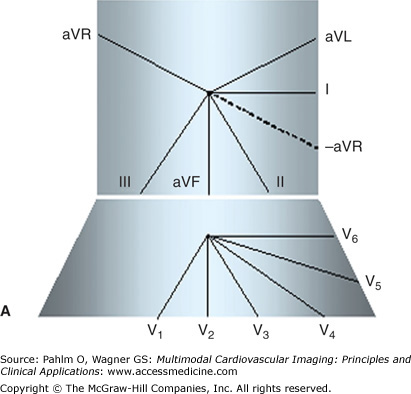
A. The scheme of the hexaxial coordination system of the standard 12-lead electrocardiogram (ECG). B. The short axis view (right) and long axis (left) view of magnetic resonance imaging (MRI). The mental three-dimensional image that would include the structural (MRI) and functional (ECG) characteristics of the heart and their temporo-spatial relations is too complicated.
Vectorcardiography partially reduces these problems. It presents the distributed electric field at every instant of time by a dipole—the equivalent dipole. This dipole is represented by a vector, defined by its magnitude and orientation, theoretically corresponding to the extent of the activation front and its location. The origin of the dipole is fixed in the center of an orthogonal coordinate system, and the trajectory of the end point of the vector during the atrial/ventricular depolarization and repolarization depicts the spatial vectorcardiographic loop. The classical graphical presentation of vectorcardiography is the planar vectorcardiogram—the planar projection of the spatial vectorcardiographic loop onto three perpendicular planes: the frontal, sagittal, and horizontal (transverse) planes.
Compared with the standard 12-lead ECG, the orthogonal ECG does not contain redundant information. The coordinate system of the orthogonal ECG/vectorcardiogram may be aligned with the geometry of the heart and to our knowledge about the sequence of atrial and ventricular activation. These characteristics make the vectorcardiogram instrumental for teaching the principles of ECG diagnosis, as well as for comparative studies with other imaging methods. However, the interpretation of vectorcardiograms is demanding for three-dimensional imagination and for good orientation in the anatomic structures and their relationships to the processes in the heart. In addition, these graphical presentations—scalar tracings of orthogonal ECG and planar vectorcardiogram—are not directly comparable with images of the heart developed from another imaging method.
In this chapter, we describe a method for graphical presentation of the orthogonal ECG/vectorcardiogram that allows the visualization of the vectors representing the cardiac electrical field comparably to other imaging methods used in cardiology. This graphical presentation of ECG is suitable for side-to-side comparisons as well as for superimposition or fusion of information from multiple imaging modalities.
In dipolar electrocardiotopography (DECARTO), the orthogonal ECG is transformed to areas projected on a spherical image surface. The original DECARTO model2,3 was developed for the presentation of the QRS complex (ie, for the process of ventricular depolarization).
The mathematical model of the DECARTO transformation is based on modeling of the cardiac electrical field. A detailed description of the electric field of the excitable myocardium would require a highly complex electrodynamics model that could link the heart as electrical generator with its electrical field. In general, outputs from electrodynamics models of the heart are ill posed in relation to the structure of the cardiac generator. It means that the given distribution of the electric field around the cardiac generator can be attributed to different generators’ shapes and/or spatial structure. This fact provides an opportunity to substitute a real source of the cardiac electrical field with a functionally equivalent generator with known compositions.4
The electrical generator of the cardiac electric field can be effectively approximated by double layers of current sources with an approximately constant density of electrical dipoles that are bounded by closed contours on the inner and outer surfaces of the ventricles. The electrostatic potential in the proximity of a double-layered object may be, in principle, calculated with any accuracy by the method of expansion in a convergent electrical multipole series describing distributions of dipoles over the double layers. The final potential is then determined by the sum of this multipole expansion.5 The number of used multipole components in the expansion depends on the required accuracy of the potential field description. The DECARTO model is based on the double-layer representation of the field generator and uses dipole representation with minimal number of multipole components. Another simplification of the DECARTO model is the assumption that the inner and outer surfaces of the heart ventricles have a spherical form, so the double layer has a spherical shape and represents so-called image surface.
The basic principle of DECARTO transformation is based on the consideration that the electrical field of the generator is formed exclusively by the electrical dipoles of the double layer and delimited to its area. This activated area is projected onto the surface of a sphere called the imaged surface. The point of intersection of the vector with the image surface is considered to be the center of the activated area. Around this point, a circle with a radius proportional to the spatial magnitude of the instantaneous vector is drawn encompassing all activated elements. In particular, the radius r of the activated area is computed for a given instantaneous spatial vectorcardiogram (VCG) vector according the following formula:
where D represents the length of the instantaneous spatial VCG vector, Dmax is the maximal spatial vector during the QRS duration, and Rs is the radius of the image sphere (Rs can be set arbitrarily; the DECARTO model uses the value of 1) (Fig. 11–2).
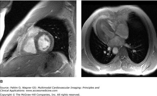
Figure 11–2.
The basic principle of the dipolar electrocardiotopography (DECARTO) method. The ventricular surface is represented by a spherical surface, the so-called image surface. The origin of the QRS vector is located in the center of the image sphere, and the intersection of the spatial QRS with the image surface gives the center of the area of activated points. The radius of the area of activated points is proportional to the maximum spatial vector magnitude.
The activated area or activated points representing this area on the image sphere are graphically presented as maps—so-called decartograms. Visualization of ventricular activation can be performed by a series of decartograms calculated and displayed individually for discrete time points or by using summary maps where activations at given time points are superimposed onto one decartogram.
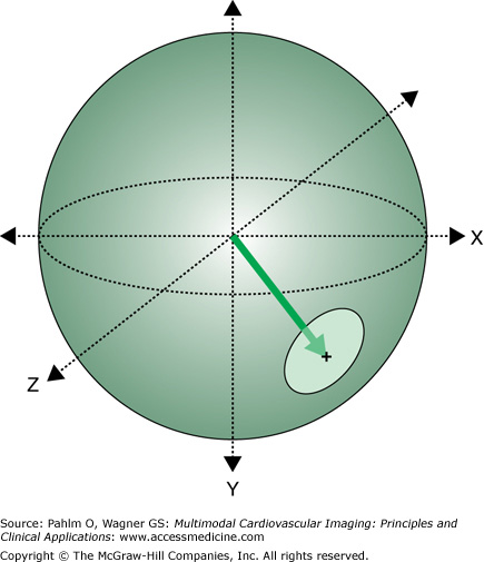
The image sphere is a hypothetical surface that represents the cardiac generator, and the activated areas on this image surface (decartograms) can be visualized by projecting them on a variety of shapes in two or three dimensions (Fig. 11–3). The selection of geometrical shapes aims to optimize the topographic relations of the abstract representations of the cardiac electric field to the activation process in the myocardium. Determination of the spatial localization of instantaneous vector end points enables the bridging between characteristics of myocardial activation propagation in this conceptual model and abstract representation of the cardiac electric field.
The spherical image surface can be easily transformed to any suitable analytical spatial or planar surfaces to visualize decartograms, such as polar (azimuthal) planar projection, rectangle projection, spherical projection, and parabolic projection, as well as to real heart surfaces rendered from other imaging methods.
The DECARTO method of graphical presentation extends the possibilities for presentation of the normal values of ECG and for its quantitative analysis. Areas of occurrence of the activated points in the normal population for decartograms were reported for the McFee-Parungao and the Frank lead systems.6 They were constructed by indicating the areas of activation at given points of QRS duration, and the probability of being activated at the given point of time for every point of the matrix was computed. In this way, reference probability matrices of normal activation were constructed (Fig. 11–4).
Figure 11–4.
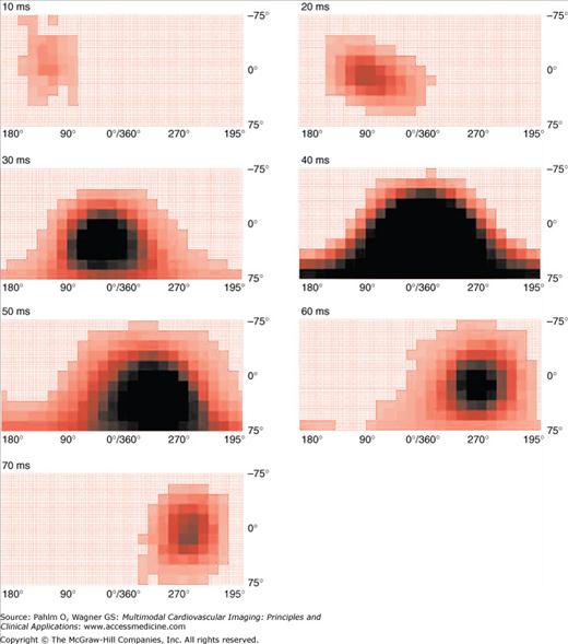
Areas of normal distribution of activated points for the Frank lead system, presented as rectangular decartograms for 10-ms intervals of QRS duration. The areas of activated points move during the QRS complex from the anterior middle part of the chest leftward and posteriorly. The decartograms were not corrected for the position of the heart in the chest; in this arrangement they are visually comparable with the body surface potential maps. The darker areas represent areas with higher probability of the occurrence of the activated points in the normal population.
Ruttkay-Nedecky7 used these probability matrices of normal activation for application of fuzzy mathematics to quantify the normality of the QRS complex. In this method, the subset of elements in the spherical surface is regarded as a fuzzy subset with membership characteristic functions derived from objective probabilities computed for the reference sample of normal subjects. In an individual case, the difference between the sum of membership function values and the mean of the reference sample at any instant of the QRS duration, or during the whole QRS, divided by the standard deviation quantifies the deviation from the reference mean value.
A similar approach was used for graphical presentation of the location and extent of the myocardium at risk in patients with acute myocardial infarction.8 This method is based on the processing of ST-segment deviations of standard 12-lead ECG following the lines set by the DECARTO method. In this ST-DECARTO method, the center of the location of the area at risk is given by the spatial orientation of the resultant spatial ST vector, and the extent of the area at risk is derived from the Aldrich score.10 The areas at risk are projected on a spherical image surface. On this image surface, a texture of the anatomic quadrants of the ventricular surface and the coronary artery supply are projected. The initial testing showed that the method allows a graphical presentation of estimated area at risk using clinically defined diagnostic rules. The area at risk can be displayed in images that are familiar for clinicians and can be compared with or superimposed on results of other imaging methods used in cardiology.
Imaging Cardiac Pathophysiology Using DECARTO
As mentioned earlier, the vector principle is the basic principle in the interpretation of ECGs. It follows that, in principle, the DECARTO method is applicable in any cardiac pathology. However, the most illustrative is the application in pathologies characterized by changes of the instantaneous spatial vector orientation. Here, we present examples of the application of DECARTO in visualizing the QRS changes in myocardial infarction and of the modified ST-DECARTO method for visualizing the area at risk based on ST-segment deviations.
Acute myocardial infarction (MI) and resulting fibrosis (scars) create regions of altered conduction. The typical signs of MI in the standard 12-lead ECG are pathologic Q waves observed in leads related to the MI location. In the VCG, the signs are manifested as changes of the instantaneous QRS vector orientation and magnitude. In decartograms, the changes in orientation and magnitude of instantaneous QRS are visible as dislocations of activated areas when compared with the normal sequence of depolarization. Figure 11–5 shows examples of instantaneous decartograms in anterior and inferior MIs and their visual comparison with the sequence of depolarization in a healthy subject.
Figure 11–5.
Decartograms in myocardial infarction using the polar projection. A. The description of the quadrants. The center of the polar projection represents the apex, and the outer circle represents the base of the ventricles. B. Series of instantaneous decartograms showing the sequence of activated areas in a normal subject in 10-ms intervals of QRS duration. C. Sequence of activated areas in a patient with anteroseptal myocardial infarction. The maximum differences are seen in the 10th and 20th ms of QRS duration; the activated areas are projected posteriorly. D. Sequence of activated areas in a patient with inferior myocardial infarction. The maximum differences are seen from the 20th and 40th ms of QRS duration; the activated areas are projected upward onto the basal segments.
The quantitative evaluation of decartograms using the fuzzy set mathematics was presented in 1994 by Ruttkay-Nedecky and Riecansky9 in patients with coronary heart disease. They recognized the following five classes of ventricular activation taking into account the locations of the activated points with respect to the normal areas: abnormal; abnormal with normal component; normal with abnormal component; marginally normal; and normal. Thus, they demonstrated the possibility to quantify not only the abnormal decartograms, but also borderline location of the activated areas.
ST-segment deviations in patients with acute MI (AMI) are associated with the location and extent of myocardium at risk, with severity of acute transmural ischemia, and with clinical outcomes.10-14 Additionally, early resolution of ST-segment elevation correlates with myocardial salvage and better prognosis in patients with AMI treated with reperfusion therapy.15-19
In practical ECG diagnostics, the location of the area of myocardium at risk is estimated from the presence of ST-segment elevation and/or depression in particular leads of the 12-lead ECG.20 For the quantification of the estimated extent of the area at risk, several formulas have been reported10,21,22
Related posts:


Stay updated, free articles. Join our Telegram channel

Full access? Get Clinical Tree


