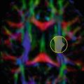
Fig. 11.1
In vivo illustration of a single streamline created in the corpus callosum, superimposed on the principal orientation field. The seed point is denoted by an asterisk. Image created with ExploreDTI software [8]
Certain criteria are required to generate anatomically plausible tracking results. Tracking is terminated once a voxel is reached that is unlikely to belong to the bundle of interest. A curvature threshold prevents sharp bending of a tract and possible propagation in an adjacent bundle. Thresholding on fractional anisotropy (FA) limits tracking to white matter regions where FA is higher. Curvature thresholds of between 30 and 70° are typically used (examples are illustrated in Fig. 11.2), while FA is typically limited to values >0.2 (as can be seen in Fig. 11.3) [9]. Parameter values are best empirically chosen, balancing between false positive and negative tracking results and accounting for the complexity of the structure. By starting at more conservative values and slowly proceeding to a more liberal regime, optimal parameter values may be determined empirically. Importantly, when multiple datasets or tracking results need to be compared, identical settings must be applied to avoid a biased result.
Fig. 11.2
Effect of the curvature threshold on the reconstruction of highly curved U-fibres (language pathways). No single optimal curvature threshold exists, the optimal value depends on the tract of interest and software and must be heuristically determined. In this case, 40° or 50° may be chosen
Fig. 11.3
Effect of the FA threshold on the reconstruction of the left corticospinal tract. A low threshold of FA = 0.1 results in more cortical tract with the cost of false positive tracts (indicated by the red arrow), which may be removed using an addition AND-ROI. A high FA = 0.3 threshold appears to be too strict, with only few tracts remaining (see the red arrow). A threshold of FA = 0.2 is considered optimal and is commonly adopted for most bundles
Additional masking may be applied to restrict tracking to specific regions. Most algorithms allow a minimal and maximal tract length to be set, as well as a seed point density , i.e., multiple seed points per voxel.
Data Requirements
Reliable tractography can only be obtained in data of sufficient quality. A correct setting of specific scanning parameters of the diffusion weighted imaging protocol is therefore crucial. The spatial resolution and the sensitivity of orientation encoding (specified by the b-value [10]) must be sufficiently high for accurate tract reconstruction, with minimal systematic errors. In addition, a high signal-to-noise ratio (mainly determined by the field strength, coil design, number of gradient directions, and parallel or multiband imaging settings) ensures that the tracking will be precise, with minimal variation. We will now discuss critical parameters and their influence on tract reconstruction.
Resolution
Diffusion-weighted MRI is limited by a relatively low spatial resolution, compared to other MR modalities. At 3 T, a resolution of 2 mm in- and through-plane can reasonably be achieved. In initial work on multislab imaging, higher isotropic resolutions of 1.3 mm [11] and 1 mm at 7 T [12] were reported.
The low resolution has a number of limiting factors on tractography. First, most white matter bundles have a thickness of only a few millimeters resulting in a coarse sampling and partial voluming. As a result, one voxel may constitute of two or more adjacent but perpendicular tracts. It was shown that up to 70 % of white matter voxels contain fibre crossings [13]. Estimating the principal diffusion orientation is then no longer possible using the diffusion tensor model. This problem was recognized more than a decade ago [14] and is known in the field as the “crossing fibre ” issue. In practice however, it refers not just to configurations where fibre tracts literally cross, but several other configurations where bundles fan, bend or “kiss.” This problem and solutions to overcome it are introduced below and covered in more detail in Chap. 21.
Second, the low resolution limits the maximum curvature of a tract that can be reconstructed. U-fibres or other connections between gyri curve over 180° within the distance of a few voxels (see Fig. 11.2). A tract thus needs to propagate by steps of 45° or more between adjacent voxels. Such strong bends may easily be ignored by tracking algorithms in favour of continuous straight connections. In addition, the chance of false positive tracking results increases by applying a liberal curvature threshold. This manifests as tracts “stepping over” or “jumping” between different adjacent bundles. A careful ROI placement is essential for accurate tract selection (see Fig. 11.4).
Fig. 11.4
False-positive tracking result. The white arrows point to crossing fibre regions where incorrect modeling results in corticospinal fibres traversing via the corpus callosum, contralaterally to the cortex. Anatomical prior knowledge is a prerequisite for correct tracking results
Tracking algorithms require data to be acquired at isotropic resolution, i.e. identical along all three axes. Data generated with sufficient in-plane resolution but a higher slice thickness does not support accurate tract reconstruction, as illustrated in Fig. 11.5 [15]. Given the current hardware supplied by most vendors, an isotropic voxel size of 2.0–3.0 mm is recommended [16].
Fig. 11.5
The effect of anisotropic resolution on tractography: an increased slice thickness from 2 to 6 mm with a constant in-plane resolution of 2 × 2 mm introduces voids in the body of the corpus callosum (top, white arrow) and reduces the tract volume in the right uncinate fasciculus (bottom)
b-Value
The strength of diffusion weighting as quantified by the b-value (Chap. 3), should be sufficiently high for a precise orientation estimation. Although a low b-value of 600 s/mm2 enables the reconstruction of large, uniform white matter tracts (see Fig. 11.6), a value of b = 1000 s/mm2 is advised for obtaining reliable results in the majority of bundles [17].
Fig. 11.6
Tracking in a dataset with a lower b-value of 600 s/mm2. The uncinate fasciculus can be accurately delineated in this dataset
In case of crossing fibre tracts, an even stronger diffusion weighting is required to unravel multiple diffusion orientations within one voxel (see Fig. 11.7). In simulations it was shown that increasing the b-value from 1000 to 3000 s/mm2 reduced the minimally resolvable angle from 45° to 30° [20]. In addition to acquiring data at a higher b-value, a higher order diffusion model must be employed to resolve crossing fibres. Multi-tensor models and constrained spherical deconvolution (CSD) are examples of approaches to this problem [19, 21, 22] (Chap. 21).
Fig. 11.7
Tractography through fibre crossings in a patient with abnormal pathway development in the pons [18]. In addition to non-diffusion-weighted images, 92 gradient directions with a b-value of 1600 s/mm2 were acquired. Deterministic tractography with a constrained spherical deconvolution (CSD) clearly shows crossing pathways [19]. Tracking performed in ExploreDTI software
Increasing the b-value reduces the measured signal value such that multiple signal averages need to be acquired, or sequences with more gradient directions must be chosen, to achieve sufficient data quality for performing reliable tractography (Chap. 6).
Gradient Directions/Signal Averages
DWMRI measures diffusion in a limited number o f orientations, which are combined to estimate an arbitrarily oriented diffusion profile. Still, the angular resolution depends on the number and configuration of the gradient directions chosen. Figure 11.8 illustrates that the uncertainty in the estimated orientation decreases when increasing the number of gradient directions from 12 to 46. Unbiased tractography requires an optimal distribution of gradient directions over the unit sphere [23]. Different methods exist for doing so, e.g., by tessellations of an icosahedron [24], or a distribution of charges. Some vendors provide predefined sets of gradient directions of different numbers (e.g., 12, 32, or 64 directions). Note that these sets may not be optimized for tractography, in which case, if possible, a user-defined gradient set should be entered.
Fig. 11.8
Cones of uncertainty of the estimated diffusion orientation superimposed on the FA of a sagittal slice through the cingulum (cing) and corpus callosum (CC) for datasets with 12 and 46 gradient directions (n g). Notice increased uncertainty for n g = 12 and in voxels with low FA
Theoretically, six directions are required to estimate the diffusion tensor. Practically, more directions are chosen for improved precision in the estimation. In Fig. 11.9, the uncinate fasciculus can be tracked with at least 24 gradient directions. In literature, a minimal set of 30 gradient directions is advised [23], while 60–80 directions are recommended for minimal variance in tractography [16].
Fig. 11.9
Tractography of the uncinate fasciculus (UF) for increasing number of gradient directions. With the theoretical minimum of six directions, the UF cannot be reconstructed
In addition, the number of signal averages (NSA) can be increased. Note that both doubling the number of gradient directions and choosing NSA = 2 increase scanning time by a factor of 2. Generally speaking, a higher number of gradient directions slightly increases the angular resolution and is preferable over multiple signal averages. Clearly, if time permits choosing NSA = 2 will improve the tracking precision even more. However, increasing the scanning time also increases the likelihood of motion artifacts, which may detract from the image quality gain achieved by increasing the NSA.
Field Strength
Imaging a t higher field strengths increases the measured signal, which in turn reduces the uncertainty in the estimated diffusion orientation. A field strength of 3.0 T is currently common practice in tractography-based clinical research studies. Tractography can successfully performed at 1.5 T, e.g., by acquiring two signal averages (NSA = 2), acquiring data along a greater number of diffusion gradient directions and by using multichannel phased-array head-coils (see Chap. 6). In a prospective evaluation of the depiction of fibre tracts at 1.5 and 3.0 T, higher visual scores, larger numbers of fibres, and a higher asymmetry index in the CST were obtained at 3.0 T [25].
High-field scanners (7.0 T and above) enable smaller anatomical structures to be identified [12]. Diffusion-weighted imaging at 7.0 T compared to 1.5 and 3.0 T showed an increased SNR that was larger than what could be expected from field strength alone: improved receive coil hardware largely contributes to higher image quality [26].
As a downside, imaging artifacts will have a higher impact at higher field strength. Inhomogeneities of the static field (B 0) spatially distort the images. Increasing the acceleration factor partly compensates this effect. Additionally, variations in the radiofrequency field (B 1) increase signal heterogeneity at 7.0 T [27].
Tract Selection
In tractography, prior anatomical knowledge on the trajectory of the bundle of interest is indispensable. Based on this knowledge, one of more regions of interest (ROIs) through which a bundle traverses need to be defined. By means of logic combinations, a set of fibre tracts representing the bundle can be obtained. See Section 4, “DTI Tractography Atlas” for further details on how to track specific white matter bundles.
Seeding
Fibre tracking is initiated from so-called seed points (see Fig. 11.1). These points may be manually annotated by the user in a single voxel or ROI. A drawback of this approach is that fibre tracking is a non-commutative procedure [28], meaning that tracking from a tract end point will not automatically result in a pathway back to the initial seed region, as is illustrated in Fig. 11.10. An alternative approach to single ROI seeding is whole-brain tractography , in which an algorithm initiates seeding in all voxels that satisfy certain criteria, e.g., all white-matter voxels with FA > 0.2 act as seed points, as displayed in Fig. 11.11. From this whole-brain tractography, the user can select a set of tracts using an ROI. The advantage of this approach is its symmetry, whereby tracts starting in the ROI and tracts from other brain regions passing through the ROI are found. This does not result in commutative tracking, but will at least result in a more robust tracking of separate branches (see Fig. 11.12). If whole-brain tractography is not supported or practically cumbersome such as in probabilistic tractography (see “Tract Selection”), multiple seed ROIs in all possible branches need to be defined as will be explained in the next section.
Fig. 11.10
Illustration of the non-commutative property of fibre tracking: seeding from the end voxel of the left tract results in a different pathway
Fig. 11.11
Whole-brain tractography (sagittal view), obtained by seeding from all voxels with FA > 0.2, colored red on the left image
Fig. 11.12
Different seeding strategies: (a) single-seed ROI versus (b) whole-brain tractography , in which case all brain white matter voxels serve as seeds. A more dense tracking is obtained using whole-brain tractography. One sagittal ROI was drawn in the body of the corpus callosum (not shown)
Logic Combination: OR/AND/NOT
Logic combi nation applied to multiple ROIs is commonly needed to delineate a bundle. The OR-operator on two ROIs returns fibres traversing through one or two ROIs. Applying the AND-operator is stricter and only returns fibres passing through both ROIs (see Fig. 11.13 for an example). The NOT-operator, removing fibres entering a specific ROI, must be used sparingly to obtain a reproducible tracking result.
Fig. 11.13
Accurate delineation of a longitudinal fasciculus . A single-seed ROI (a) results in many false positive fibres (b). Adding a second AND ROI (c) removes these fibres from the selection, resulting in the desired pathway
Good Practice for ROI-Drawing
Tractography requires spatial awareness and interpretation of a 3D representation on a 2D screen (although some packages support stereo-viewing). Hence it requires a number of trial-and-error experiments before an accurate result is achieved. Direct feedback from the software aids in speeding up the training phase. A number of programs support interactive exploration, providing instant tracking results after the user updates selection regions. There are currently methods available, which allow interactive positioning of a single seed point or one or more selection boxes (Fig. 11.14).
Fig. 11.14
Interactive tractography of the cingulum bundle using two boxes. Transparent colored fibres reflect fibres originating from the corresponding box. Solid green fibres represent the cingulum tract, connecting both boxes. Image created with DTI interactive (DTIi) software [29]
More accurate tracking may be achieved by delineating arbitrarily shaped ROIs on anatomical scans. The fractional anisotropy (FA) map color-coded for orientation provides a good reference for annotation. Essentially, this map encodes all information employed during tracking. Most accurate tracking is achieved by annotating on a plane perpendicular to the (local) tract orientation. The color information aids the user to identify such a plane. Including low-intensity voxels representing low FA will not affect tractography, since these voxels are automatically disregarded based on an FA threshold by the algorithm (see Box 11.1)
Box 11.1: On Estimating Tract Volume and FA (Consideration Box for Researchers)
In a research study, there may be hypotheses of microstructural damage, resulting in reduced FA in a tract or white matter atrophy resulting in reduced tract volume on macroscopic level. Figure 11.15 shows results of a tractography training session of students and suggests that tract volume is measured with less precision compared to the mean FA within a tract, considering the large variation in the number of obtained voxels by the students. Indeed, in literature larger variations in tract volume than tract FA were reported [59]. This work also showed that traumatic volume loss confounds FA estimates, since FA was reduced in smaller volume tracts, likely caused by partial volume effects. Including tract volume as covariate in the statistical model is one way of overcoming this issue [60].
Fig. 11.15
Results of a training session of a group of 15 students. (a) Mean FA and number of voxels of two tracts created by the students. (b) Illustrative image of a correct tracking of the Forceps Major, containing approximately 4000 voxels. Tracking performed in DTI-Studio software [30]
Be aware that annotating ROIs on the FA map may create a bias, since the ROIs are drawn on the same maps that will be used for statistical comparison.
A high-resolution structural scan provides additional anatomical reference and can be used in addition to the color-coded FA map. One must keep in mind that the spatial resolution of the diffusion data is commonly a factor of two lower. Also, it is necessary to verify that the scans are spatially aligned and a correction for possible head motion will typically be needed. In addition, a spatial distortion correction of the diffusion data may be required by means of acquiring a B 0-map or performing nonrigid registration (see Chap. 7).
The tractography result is dependent on the selection criteria as imposed by the user. Procedures for reproducible reconstruction of major white matter tracts with deterministic tractography have therefore been proposed [31]. Even when following synchronized tracking procedures, the inter-observer agreement in practice has been reported as not exceeding 90 % [32]. This means that some variability exists in the tract volume obtained from ROIs drawn by different users. This variability is illustrated in Fig. 11.15, summarizing a training session in which students were assigned to reconstruct the forceps major and cingulum tracts. Large variations in tract volume are observed, resulting from differences in ROI size and positioning. One can conclude that training on multiple datasets is required to converge to reproducible findings. Also note that the inter-observer variability in average FA is relatively low.
The following guidelines may aid in achieving a reproducible tracking:
Draw ROIs as large as possible. This may seem counter-intuitive, but ensures that any possible fibre belonging to a bundle will be included.
Annotate 2D ROIs in the plane perpendicular to the bundle orientation.
Apply as few ROIs as possible. In most situations, two or three ROIs suffice, i.e., one OR ROI at one end of the tract, an AND ROI at another end and another AND ROI along the pathway to exclude any deviating tracts.
Use NOT-ROIs sparingly. Only fibres appearing as clear outliers may be removed.
In case whole-brain tractography is unavailable, generate two overlapping seed and AND ROIs at both sides of a tract. By doing so a symmetric tracking result is obtained (see Fig. 11.17).
Section 4 of this book discusses normal anatomy described by a DTI atlas.
Probabilistic Tractography
The principal orientation of diffusion can only be estimated with a certain limited precision [33]. The uncertainty increases both with higher noise levels or fewer gradient directions and lower diffusion anisotropy (see Fig. 11.8).
Tractography is highly sensitive to uncertainty in the orientation estimation. By each tracking step into an adjacent voxel, the pathway will further deviate from the truth. In other words, the uncertainties propagate or accumulat e, such that tracts may terminate prematurely and the target pathway may not be found. One must be aware that this uncertainty is invisible in conventional deterministic tractography visualizations, which tend to be perceived as precise segmentation while in reality this may not be the case, as is illustrated in Fig. 11.4.
Fortunately, knowledge on the amount of uncertainty in the orientation estimation can be used to obtain potentially precisely delineated pathways. Tractography as it has been introduced thus far is characterized as deterministic. Repeated tracking instances from a single seed point will return identical tracking results, based on an average orientation estimate per voxel (Fig. 11.16).
Fig. 11.16
Deterministic and probabilistic tractography. (a) Deterministic tractography is based on the principal eigenvector, while probabilistic tractography is based on a distribution of estimated possible orientations. (b) From a seed voxel, a single tract is computed in deterministic tracking. Probabilistic tracking proceeds along one randomly selected orientation per voxel. (c) After probabilistic tracking, a tract probability map is computed for the relative number of tracts passing through a voxel
Probabilistic tractography instead estimates the orientation distribution in each voxel [21, 34] (see Fig. 11.8). The mean of this distribution equals the orientation used in deterministic tractography. The width of the distribution is proportional to the uncertainty. Once the distribution is known, multiple tracts in the order of 10,000 are seeded from each seed point. A tract is computed on an orientation estimate drawn from the distribution in all voxels. Each tract thus follows a different pathway. From the average number of visits of the tracts to each voxel, a tract probability map can be derived. When the orientation uncertainty is low, all tracts will traverse along a similar pathway. Tracts passing through a single area with high uncertainty will spread and show a diffuse pattern afterwards.
Related posts:

Stay updated, free articles. Join our Telegram channel

Full access? Get Clinical Tree


