Introduction
Since the 1950s when Edler and Hertz1,2 in Lund, Sweden, recorded ultrasonic images of the heart walls and normal and rheumatic mitral valves, echocardiography has assumed a central role in the diagnosis and management of most cardiac disorders.
The purpose of this chapter is to examine the role of modern echocardiography from the perspective of the general practitioner. After a brief summary of the salient technical aspects of echocardiography and the elements of a normal echocardiographic examination, 10 clinical vignettes will be presented to illustrate the central role of echocardiography in contemporary medicine.
Physics
Sound is a mechanical phenomenon involving the transfer of energy through a medium. Ultrasound occurs in nature as illustrated by certain bat species that use ultrasound to navigate and to identify prey. The dog whistle is an example of a simple man-made ultrasound device.
A sound wave is generally depicted as a sine wave. Sound is defined by its amplitude, wavelength (λ) (the distance between cycles), and its frequency (f), the number of cycles in a given period of time (Fig. 1–1). Velocity (v = f × λ) is the speed at which a sound wave travels through a particular medium or body tissue. Velocity is dependent on the physical properties of the tissue and its acoustic impedance, which is primarily determined by the tissue’s density.
The frequency of a sound wave is measured in hertz (Hz). One cycle per second is 1 Hz. Ultrasound is sound above the audible range, having a frequency greater than 20,000 cycles per second (20 kHz). In clinical medicine, transducers create ultrasound waves with much higher frequencies, ranging from 2 to 15 MHz. Higher frequency transducers give superior near-field resolution but have less tissue depth penetration.
A sound wave will travel in a relatively straight line through a homogeneous medium with some attenuation due to absorption and scatter until it reaches an interface between media with different densities. At the interface, the sound wave will undergo reflection and refraction proportional to the different densities of the two tissues (Fig. 1–2).
Modern commercial ultrasound systems are comprised of three basic components: a transducer that serves as a sound originator and as a receiver, a computer, and a display monitor. The ultrasound transducer contains piezoelectric elements, which were originally quartz but are now complex ceramics.
The piezoelectric effect was described by the brothers Jacques and Pierre Curie in 1880.3-5 The brothers discovered that mechanical stress caused certain crystals to alter their shape and produce an electrical charge proportional to the mechanical stress (Fig. 1–3). This property is now referred to as reverse piezoelectricity. Commercial uses of piezoelectric elements include the igniters in gas grills and triggers for automobile air bags.
Piezoelectric elements also have the property of changing shape when placed in an electric field creating ultrasonic sound waves (Fig. 1–4). When functioning as a transducer as part of an ultrasound system, the piezoelectric elements are placed in an electric current, causing them to change shape and emit an ultrasonic wave.
Modern phased array ultrasound transducers contain several thousand piezoelectric elements that are focused electronically. This allows for some of the piezoelectric elements to transmit sound waves, while other elements are simultaneously receiving the returning sound waves, thereby creating continuous wave systems.
When functioning as a receiver of the reflected sound waves, the echoes, the piezoelectric elements change shape and create electrical pulses. The computer signal processor knows the amount of time from the moment that the transducer emitted the ultrasonic wave until it received the returning echo sound wave. Knowing the speed of ultrasonic waves through tissue (sound travels through water, the primary constituent of human soft tissue, at approximately 1540 m/s), the computer can then calculate the distance of the reflecting tissue from the transducer (Fig. 1–5).
Figure 1–5.
Distance calculations. Echocardiographic method of determining an object’s distance from the transducer. In this example, the object is 1 meter from the transducer as calculated from the time for the transmitted sound wave to strike the distant object and be reflected back to the transducer. The distance information is used to construct structural images.
Although the electronics are complex, the principles are simple. With this distance information, the computer creates visual analog or digital displays. Displaying the points over time allows for the graphic depiction of the heart, creating M-mode (time motion), and two-dimensional echocardiograms (Fig. 1–6).
In 1842, the Austrian mathematician, Christian Doppler, presented a treatise entitled “On the Colored Light of Binary Stars and Certain Other Stars of the Heavens,” in which he postulated that the perceived color of the light waves emanating from stars was affected by the motion of the stars. In 1845, the Dutch chemist and meteorologist Buys Ballot demonstrated the acoustic principles of the Doppler effect in a now classic experiment using musicians on a moving train to explain the perceived changes in a sound’s pitch when it is emitted from a moving source.6 To the stationary observer, the sound appears to increase in frequency (pitch) as the source approaches due to compression of the sound wave and to diminish in frequency as the source recedes (Fig. 1–7).
In echocardiography, the Doppler effect or shift is the difference between the frequency of the original transmitted sound wave compared with the frequency of the received sound waves caused by the motion of the reflecting tissue. The computer measures the Doppler shift and then uses this information to calculate the velocity of the moving reflecting target. In cardiac Doppler, the moving target has been red blood cells. Therefore, the Doppler shift can be used to provide the indirect assessment of the direction and velocity of blood, which in turn serve as the basis for echocardiographic-derived hemodynamic measurements. More contemporary tissue Doppler techniques assess the movement of actual cardiac structures, for example, the mitral valve annulus.
An important practical point in clinical ultrasound imaging is that the angle between the transmitted sound waves and the path of the moving target is critical to the mathematical calculations. The more parallel the transmitted ultrasound is to the moving target, the more accurate the calculation of the target’s velocity. At an angle of 90°, the Doppler shift cannot be recorded.
The opposite is true in two-dimensional echocardiography, in which the quality of the images is optimized when the structures are perpendicular to the transmitted ultrasound.
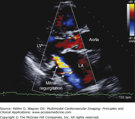
Color flow Doppler provides a spatial display of blood flow velocity and direction. This is accomplished by having the transducer simultaneously transmit multiple sound waves in a predetermined sector. By measuring the Doppler frequency shift, blood flow velocity and direction are determined and displayed in two-dimensional space as a color map. This information is continuously updated during the cardiac cycle, providing real-time depictions of intracardiac blood flow velocity and direction. For example, a mitral regurgitant blood flow jet becomes recognizable when the Doppler color flow information is displayed superimposed on the real-time two-dimensional images of the mitral valve (Fig. 1–8).
Normal Cardiac Echo Doppler Examination
The standard cardiac echo Doppler clinical examination includes four basic transducer positions (Fig. 1–9) to obtain the following nine views:
Figure 1–9.
Transducer positions. Illustration of the four basic transducer positions for obtaining the standard transthoracic echocardiographic views. The patient is on his left side for transducer positions 1 (parasternal long axis) and 2 (apical) and flat on his back for positions 3 (subcostal) and 4 (suprasternal). Reproduced from Oh J, et al. The Echo Manual. Third Edition, 2006. By permission of Mayo Foundation for Medical Education and Research. All rights reserved.
Parasternal long axis
Right ventricular inflow/right ventricular outflow
Parasternal short axis
Apical four-chamber
Apical five-chamber
Apical two-chamber
Apical three-chamber
Subxiphoid four-chamber/short axis
Suprasternal notch
Each view typically includes a two-dimensional recording followed by M-mode, color flow, and Doppler recordings. The following sections and tables outline the cardiac structures and the most common two-dimensional and Doppler abnormalities for each of the echocardiographic views.
With the patient lying on his or her left side, the transducer is placed at the left parasternal border in the fourth left intercostal space (position 1) (Fig. 1–10; Table 1–1).
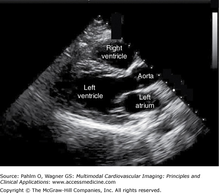
Figure 1–10.
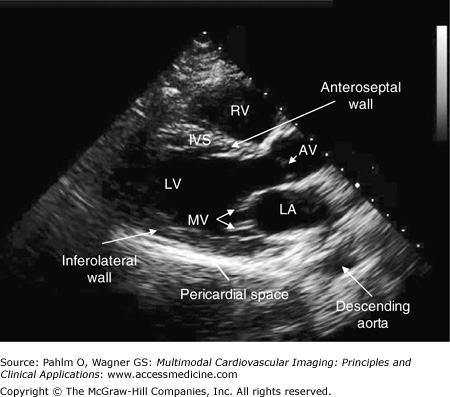
Parasternal long axis view. A parasternal long axis image is obtained with the patient lying on his left side; the transducer is positioned in the patient’s fourth left intercostal space. AV, aortic valve; IVS, interventricular septum; LA, left atrium; LV, left ventricle; MV, mitral valve; RV, right ventricle.
| Cardiac Structures | Echocardiographic Abnormalities | Doppler Abnormalities |
|---|---|---|
| Right ventricle | Dimensions Hypertrophy Ebstein anomaly Arrhythmogenic right ventricle | Ventricular septal defects |
| Aortic root | Dimensions Dissection | |
| Aortic valve | Leaflet thickness vegetations | Outflow obstruction
|
| Mitral valve | Leaflet appearance Mitral valve prolapse/flail Systolic anterior motion Mitral valve vegetations Mitral annular calcification | Stenosis Regurgitation |
| Left ventricle | Dimensions Hypertrophy Wall motion: anteroseptal and inferolateral walls | Muscular ventricular septal Defects |
| Septum | Atrial septal defects Atrial septal aneurysm | Intra-cardiac shunt |
| Pericardium | Effusion Tumors Cysts |
Without changing the transducer’s position on the patient’s chest (position 1), the transducer is tilted inferiorly and angled medially to visualize the right atrium and the right ventricle (Fig. 1–11; Table 1–2).
Figure 1–11.

Right ventricular inflow view. A right ventricular inflow image is obtained with the patient and transducer positioned as in the parasternal long axis view. The transducer is tilted inferiorly and angled medially to provide images of the right atrium, the right ventricle, and the tricuspid valve. RA, right atrium; RV, right ventricle.
| Cardiac Structures | Echocardiographic Abnormalities | Doppler Abnormalities |
|---|---|---|
| Right atrium | Dimensions Masses Chiari network Eustachian valve | Membrane in the right atrium |
| Tricuspid valve | Leaflet thickness Vegetations | Stenosis Regurgitation |
| Right ventricle | Dimensions Wall thickness Contractility |
Without changing the transducer’s position on the patient’s chest (position 1), the transducer is tilted superiorly and angled laterly to visualize the pulmonary artery and the outflow of the right ventricle.
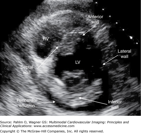
Without changing the transducer’s position on the patient’s chest (position 1), the transducer is rotated 90° clockwise, and the heart is scanned from base to apex (Figs. 1–12 and 1–13; Table 1–3).
Figure 1–12.
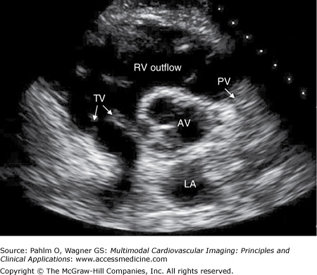
Parasternal short axis view. A parasternal short axis image is obtained by rotating the transducer 90° clockwise. Parasternal short axis views are generally obtained at the levels of the cardiac base, the mitral valve, the mid cavity, and the LV apex. This is a short axis image at the cardiac base. AV, aortic valve; LA, left atrium; PV, pulmonic valve; TV, tricuspid valve.
| Cardiac Structures | Echocardiographic Abnormalities | Doppler Abnormalities |
|---|---|---|
| Proximal aorta | Aortic valve morphology | Membranous and supracristal ventricular septal defects |
| Right venricular outflow track | Infundibular stenosis | |
| Pulmonic valve | Appearance vegetations | Stenosis Regurgitation |
| Tricuspid valve | Appearance vegetations | Stenosis Regurgitation |
| Mitral valve | Appearance vegetations | Stenosis Regurgitation |
Left ventricle:
| Wall motion: anterior; septal; anteroseptal; lateral and inferior walls |
The transducer is positioned at the patient’s apex or point of maximal impulse. The ultrasound beam is directed toward the patient’s right shoulder (position 2) (Fig. 1–14; Table 1–4).
Figure 1–14.
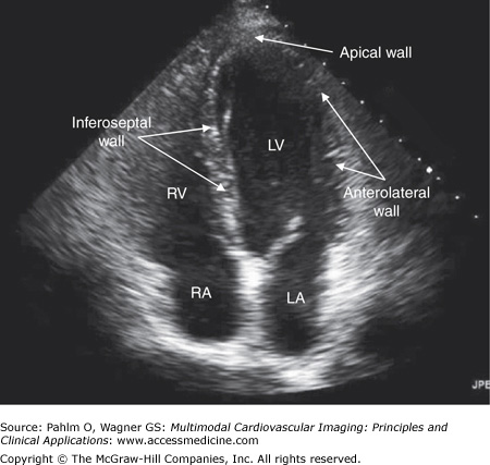
Apical four-chamber view. An apical four-chamber image is obtained with the patient lying flat or on his left side with the transducer positioned at the patient’s point of maximal impulse and directed at his right shoulder. LA, left atrium; LV, left ventricle; RA, right atrium; RV, right ventricle.
| Cardiac Structures | Echocardiographic Abnormalities | Doppler Abnormalities |
|---|---|---|
| Left atrium | Dimensions Pulmonary veins | Atrial septal defects Patent foramen ovales Pulmonary blood flow |
| Left ventricle | Dimensions wall motion: inferoseptum; apex; and anterolateral walls Aneurysms Mural thrombus | |
| Right atrium | Dimensions Chiari network Eustachian valve | |
| Right ventricle | Dimensions Arrhythmogenic right ventricle | Ventricular septal defects |
| Mitral valve | Appearance | Stenosis Regurgitation |
| Tricuspid valve | Appearance Location | Stenosis insufficiency |
| Pericardial space | Effusion Tamponade: right atrial/right ventricular collapse | Tamponade: abnormal mitral inflow respiratory variation |
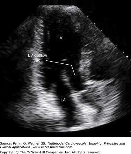
The transducer is angulated slightly anteriorly to bring the left ventricular outflow tract and the aortic valve into better definition (Fig. 1–15; Table 1–5).
Figure 1–15.
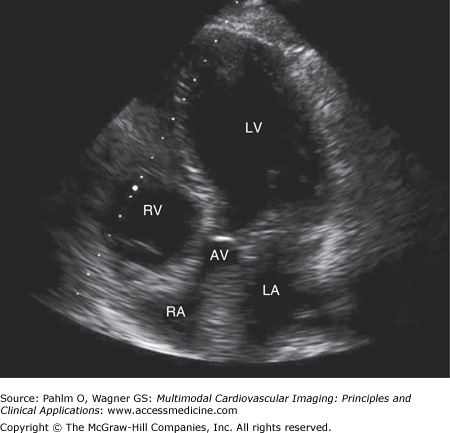
Apical five-chamber view. An apical five-chamber image is obtained with the patient and the transducer similarly positioned to the apical four-chamber view with slight anterior angulation to bring the left ventricular outflow tract into the plane of view. AV, aortic valve; LA, left atrium; LV, left ventricle; RA, right atrium; RV, right ventricle.
| Cardiac Structures | Echocardiographic Abnormalities | Doppler Abnormalities |
|---|---|---|
| Left atrium | Dimensions | Atrial septal defects Patent foramen ovales |
| Left ventricle | Dimensions Wall motion: inferoseptum; apex; and lateral walls Aneurysm Mural Thrombus | |
| Right atrium | Dimensions | |
| Right ventricle | Dimensions | |
| Mitral valve | Appearance | Stenosis Regurgitation |
| Tricuspid valve | Appearance Location | Stenosis Regurgitation |
| Left ventricular outflow tract | Sub/supravalvular membranes | Obstruction Regurgitation |
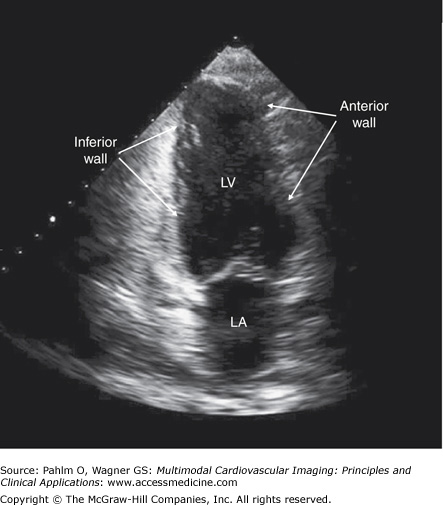
The transducer is positioned at the patient’s cardiac apex as it is in the apical four-chamber and five-chamber views, but it is rotated 90° counterclockwise (Fig. 1–16; Table 1–6).
| Cardiac Structures | Echocardiographic Abnormalities | Doppler Abnormalities |
|---|---|---|
| Left atrium | Dimensions Left atrial appendage | Atrial septal defect Patent foramen ovale |
| Left ventricle | Dimensions Wall motion: anterior; apex; and inferior walls |
The transducer remains positioned at the patient’s cardiac apex as it is in the apical four-chamber and five-chamber views, but it is rotated 180° counterclockwise (Fig. 1–17; Table 1–7).
| Cardiac Structures | Echocardiographic Abnormalities | Doppler Abnormalities |
|---|---|---|
| Left atrium | Dimensions | Atrial septal defect Patent foramen ovale |
| Left ventricle | Dimensions wall motion: anteroseptal; apex; and inferolateral | |
| Left ventricular outflow tract |
The transducer is located in the patient’s right upper quadrant directly below the xiphoid process (position 3). The ultrasound beam is directed at the patient’s left shoulder. From this position, the ultrasound waves travel through the patient’s liver, a solid structure. This will often provide superior images in patients with severe chronic obstructive pulmonary disease (COPD) or morbid obesity in whom imaging in the standard parasternal positions often provides suboptimal images (Fig. 1–18; Table 1–8).
Figure 1–18.
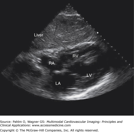
Subxiphoid/subcostal view. A subxiphoid/subcostal image is obtained with the patient lying flat with the transducer positioned below the patient’s xiphoid process. The transducer is directed to the patient’s left shoulder. LA, left atrium; LV, left ventricle; RA, right atrium; RV, right ventricle.
| Cardiac Structures | Cardiac Abnormalities | Doppler Abnormalities |
|---|---|---|
| Left atrium | Dimensions | Atrial septal defects Patent foramen ovale |
| Left ventricle | Dimensions Wall motion | |
| Right atrium | Dimensions | |
| Right ventricle | Dimensions Hypertrophy | Ventricular septal defects |
| Mitral valve | Appearance | Stenosis Regurgitation |
| Tricuspid valve | Appearance Location | Stenosis Regurgitation |
| Pericardial space | Effusion/tamponade | Tamponade |
| Inferior vena cava | Hepatic vein respiratory variation | Hepatic vein blood flow |
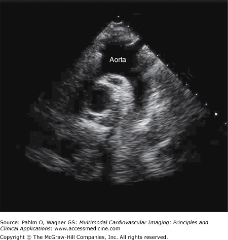
The transducer is positioned in the patient’s suprasternal notch (position 4). The ultrasound beam is directed anteriorly and to the right to image the ascending aorta and posteriorly and to the left to image the descending aorta (Fig. 1–19; Table 1–9).
| Cardiac Structures | Echocardiographic Abnormalities | Doppler Abnormalities |
|---|---|---|
| Aorta | Atherosclerosis Aneurysmal dilatation Dissection | Aortic insufficiency Coarctation Patent ductus arteriosus |
| Pulmonary artery | Dimensions Pulmonary emboli |
Assessment of Left Ventricular Systolic and Diastolic Function
The most common clinical indication for echocardiographic imaging is an assessment of left ventricular (LV) function. There are four methods of assessing LV systolic function:
- Visual inspection
- Contrast enhancement
- Regional wall motion scoring
- Quantitative methods
- Fractional shortening
- Simpson method
- Fractional shortening
An accurate assessment of LV systolic function depends on the identification of the endomyocardial surface in each of the transducer positions.
Visual inspection provides a qualitative and a semiquantitative assessment of LV systolic function LV ejection fraction (LVEF) (Table 1–10).
| Visual Assessment | Approximate Left Ventricular Ejection Fraction (%) |
|---|---|
| Increased | >75 |
| Normal | 55-75 |
| Mildly reduced | 45-55 |
| Moderately reduced | 35-45 |
| Severely reduced | <35 |
In patients in whom the endomyocardial border is not well defined, for example for patients with COPD or morbid obesity, better definition of the endomyocardial borders (ie, the LV cavity) can be obtained with the injection of intravenous contrast material. This contrast is comprised of gas-filled microbubbles or microspheres to opacify the LV chamber and thereby better define the borders, shape, and regional and global wall motion of the left ventricle (Fig. 1–20).
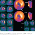
Regional wall motion scoring is a semiquantitative method in which 17 discrete segments of the LV chamber are identified, each of which is given a score (normal or hyperkinesis = 1, hypokinesis = 2, akinesis [negligible thickening] = 3, dyskinesis [paradoxical systolic motion] = 4, and aneurysmal [diasystolic deformation] = 5) (Fig. 1–21).7
Figure 1–21.
Left ventricular (LV) wall segments. The LV walls are divided into 16 segments to provide a method of semiquantitatively grading LV regional and global systolic function. LAX, parasternal long axis; 4C, apical four-chamber; 2C, apical two-chamber; SAX, parasternal short axis; MV, mitral valve level; PM, papillary muscle level; AP, apex. Reprinted with permission. Circulation. 2002;105:539-542. © 2002 American Heart Association, Inc.
The wall motion score index (WMSI) is obtained by dividing the sum of the wall motion scores by the number of satisfactorily visualized segments:
The wall motion score (WMS) LVEF is obtained by dividing the sum of the regional wall motion scores by the number of segments scored and then multiplying by 30 (normal = 2, hypokinesis = 1, akinesis = 0, and dyskinesis = -1) (Table 1–11):
| Wall Motion Score Index | Wall Motion Score Left Ventricular Ejection Fraction |
|---|---|
| 1 = Normal | 3 = Increased |
| 2 = Hypokinetic | 2 = Normal |
| 3 = Akinetic | 1 = Hypokinetic |
| 4 = Dyskinetic | 0 = Akinetic |
| 5 = Aneurysmal | −1 = Dyskinetic |
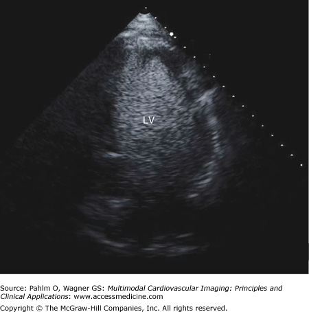
Fractional shortening is the classic M-mode method to estimate LV systolic function. The LV end-diastolic (LVED) and end-systolic (LVES) dimensions are measured in either the parasternal long axis or short axis view:
Fractional shortening is based on a single plane creating a limited “keyhole” view of the left ventricle (Fig. 1–22). Therefore, it is only useful for normal ventricles and in patients with dilated cardiomyopathies without regional wall motion abnormalities.
Figure 1–22.
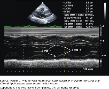
Fractional shortening. A parasternal long axis M-mode image with an end-diastolic dimension of 3.9 cm, an end-systolic dimension of 2.3 cm, and normal calculated left ventricular fractional shortening of 41.0% (normal >27%), and normal left ventricular ejection fraction of 72.5% (normal ≥55%). EF, ejection fraction; FS, fractional shortening; LVIDd, left ventricular end-diastolic dimension; LVIDs, left ventricular end-systolic dimension.
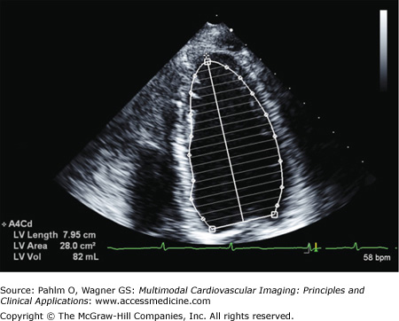
When there are regional wall motion abnormalities, the more reliable quantitative system of determining LV volumes and LVEF is based on the Simpson method (Figs. 1–23 and 1–24). In either the apical four-chamber or two-chamber view, the endocardial border is traced in end-diastole and end-systole. The LV is then divided into a number of cylinders or discs, generally 20, of equal height. Individual volumes are calculated to yield the overall LV volume and LVEF.

Diastole is an energy-dependent process with four phases:
The isovolumic relaxation time (IVRT) during which LV pressure drops but the mitral valve remains closed.
Early rapid LV filling begins when LV pressures fall below left atrial pressures and the mitral valve opens. Transmitral blood flow in this early phase is due to a combination of myocardial relaxation and elastic recoil, which in effect sucks blood into the left ventricle. The E wave depicts early diastolic mitral inflow velocity. It is a measure of LV relaxation.
The diastasis period is the mid-diastolic period during which transmitral blood flow is minimal.
End-diastole is the final phase during which there is an increase in transmitral flow resulting from left atrial contraction. In normals, approximately 15% to 20% of LV filling occurs during this phase. End-diastole is depicted by the A wave.
Doppler diastolic indices are affected by a patient’s age, heart rate and rhythm, conduction abnormalities, and the loading conditions of the heart. Figure 1–25 illustrates normal and abnormal mitral inflow diastolic filling patterns.
Figure 1–25.

Left ventricular (LV) diastolic inflow patterns. Normal and abnormal diastolic transmitral inflow and pulmonary venous flow patterns are illustrated. A, velocity at atrial contraction; a′, velocity of mitral annular motion with atrial systole; Adur, A duration; AR, pulmonary venous atrial reversal flow; ARdur, AR duration; D, diastolic forward flow; DT, deceleration time; E, peak early filling velocity; e′, velocity of mitral annulus early diastolic motion; S, systolic forward flow; *, corrected for E/A fusion. Reproduced with permission from Redfield M, et al. Burden of systolic and diastolic ventricular dysfunction in the community. JAMA. 2003;289:194-202. Copyright 2003 American Medical Association. All rights reserved.
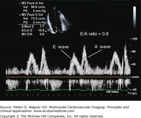
When assessing LV diastolic function, the Doppler sample volume is positioned at the tips of the mitral valve leaflets in the apical four-chamber view. Doppler measurements are made of the IVRT, the E wave, the E wave deceleration time, and the A wave (Fig. 1–26).8
Figure 1–26.
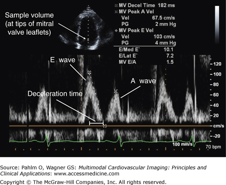
Normal left ventricular diastolic mitral inflow. With the sample volume placed at the tips of the mitral valve (MV) leaflets, a normal mitral inflow pattern is illustrated with an early rapid E wave velocity of 103 cm/s, a late A wave velocity following atrial contraction of 67.5 cm/s, an E/A ratio of 1.5 (normal >1.0), and a deceleration time of 182 ms.
Due to normally rigorous myocardial contraction and brisk LV elastic recoil, approximately 80% of LV filling occurs during the early phase of diastole. This results in the E wave velocity being 1.0 to 1.5 times greater than that of the A wave, a deceleration time >140 ms, septal E′ >10 cm/s, and E/E′ <8 (see “Tissue Doppler Imaging” below).
Due to impaired myocardial relaxation, the E wave velocity is reduced, and the deceleration time is prolonged. This results in more filling in late diastole, which is reflected in an increase in the A wave velocity and an E/A ratio of <1.0 (Fig. 1–27).
Impaired myocardial relaxation is combined with a mild to moderate increase in left atrial pressures, which results in a pseudonormalized LV filling pattern, ie an E > A wave pattern.
There are several methods of differentiating normal from pseudonormal LV diastolic function, including (1) identification of diastolic flow abnormalities in the pulmonary veins, (2) use of the Valsalva maneuver, and (3) use of tissue Doppler imaging.
Impaired myocardial relaxation combined with a marked increase in left atrial pressures causes a shortened IVRT, which results in rapid but shortened early filling as reflected by an increase in E wave velocity and a shortened deceleration time. The A wave velocity and duration are reduced because of rapidly increasing pressures in the noncompliant left ventricle. This results in a “restrictive pattern” of transmitral filling with an E/A ratio >1.5 and a deceleration time of <140 ms.
The resting transmitral filling patterns are similar to the grade 3 pattern; however, the patterns differ during a Valsalva maneuver.
The Valsalva maneuver can help differentiate between a normal filling pattern and a grade 2 “pseudonormalized” pattern seen in patients with impaired relaxation combined with a mild-moderate increase in filling pressures.
During phase 2 of a Valsalva maneuver, there is decreased venous return with a resultant decrease in the heart’s preload. If the Valsalva maneuver is maintained, there will be a resultant decrease in stroke volume and systemic blood pressure. In normals, a Valsalva maneuver will result in a decrease in both the E and A waves. Therefore, the normal E > A ratio is preserved. However, in patients with LV diastolic dysfunction and a grade 2 “pseudonormalized” pattern of their resting diastolic filling, the Valsalva maneuver will cause a decrease in the E wave and an increase in the A wave, thereby causing an abnormal A > E wave pattern and the unmasking of the diastolic dysfunction.
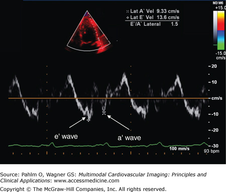
Tissue Doppler imaging focuses on the motion of cardiac structures, specifically the septal and lateral regions of the mitral annulus, to assess myocardial relaxation. The same Doppler principles are used to measure the relatively slower velocity but higher amplitude of the motion and direction of myocardial tissue in the same way that the velocity and direction of blood flow are measured.
The E′ wave velocity, when measured at the medial or septal portion of the mitral annulus, is normally ≥10 cm/s; when the E′ wave velocity is measured at the lateral portion of the mitral annulus, it is generally higher, normally ≥15 cm/s (Figs. 1–28 and 1–29).
Figure 1–28.
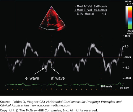
Tissue Doppler. By placing the sample volume at the medial/septal or lateral aspect of the mitral valve annulus, the relatively slower velocity but higher amplitude of the heart itself can be assessed. In this example, at the medial aspect of the mitral annulus, the velocity of the e′ wave is 10.6 cm/s, lowerset, the a′ wave velocity is 8.48 cm/s, and E’/A’ ratio is 1.3.
The E′ wave reflects myocardial relaxation. It is depressed in all stages of diastolic dysfunction. Therefore, there is no “pseudonormal pattern” seen in tissue Doppler recordings. Also, because the E wave increases with higher filling pressures, the E/E′ ratio correlates well with LV filling pressures.
Patients with normal LV diastolic relaxation and filling pressures will a have septal E′ wave velocity >10 cm/s and an E/E′ ratio of <8. Patients with grade 2 pseudonormalized LV filling patterns will have an E′ wave velocity of <7 cm/s and an E/E′ ratio of >15 due to their increased filling pressures.
For patients who are unable to exercise, dobutamine stress echocardiography is a clinically useful alternative to pharmacologic nuclear stress testing. Unlike the vasodilating agents used in nuclear imaging, dobutamine stimulates the adrenergic receptors causing an increase in myocardial contractility, heart rate, and blood pressure and, as a consequence, an increase in myocardial oxygen demand.
Related posts:
 Optical Mapping of Electrical Activity
 Phonocardiography
 Ischemic Heart Disease
 Development of the Heart, with Particular Reference to the Cardiac Conduction Tissues
 Myocardial Perfusion Single Photon Emission Computed Tomography and Positron Emission Tomography
 Cardiac Magnetic Resonance Imaging in Ischemic Heart Disease
Stay updated, free articles. Join our Telegram channel

Full access? Get Clinical Tree


