Introduction
Electrocardiograms (ECGs) recorded simultaneously at many body surface sites can be used to construct a sequence of body surface potential distributions that correspond to cardiac electrical activity; this technique is referred to as body surface potential mapping (BSPM).1,2 The noninvasively acquired BSPM data can be used, in turn, along with a mathematical model that accounts for geometry and electrical properties of the thorax, to reconstruct electrical potentials on the epicardial surface. The problem of calculating epicardial potentials from recorded BSPM data constitutes one of the formulations of the inverse problem of ECG.3,4
The calculation of epicardial potentials from noninvasively acquired electrical and anatomic data is also referred to, quite aptly, as electrocardiographic imaging.5,6 The procedure requires BSPM data, accurate representation of the patient’s thoracic geometry, routines for calculating transfer coefficients relating epicardial and body surface potentials,7 and reliable inverse-solution techniques for estimating epicardial potentials from BSPM data.3,4 Patient-specific anatomic data can be obtained by computed tomography (CT) or magnetic resonance imaging (MRI). ECG imaging has shown its potential in theoretical and experimental studies,5,6 and it promises to find its way into routine clinical applications.8,9
The aim of this chapter is to illustrate the use of ECG imaging in clinical cardiac electrophysiology, in particular as an aid to radiofrequency catheter ablation of ventricular arrhythmias. In this chapter, we introduce our methodology of BSPM, with particular attention to applications in clinical cardiac electrophysiology; we deal with the mathematical formulation of the relationship between potentials on the epicardial surface and body surface and show how this relationship is used to solve the inverse problem of ECG in terms of epicardial potentials; we describe the application of ECG imaging during catheter-ablation procedures in the clinical cardiac electrophysiology laboratory; and we discusses results reported in this chapter in the context of current clinical practice.
Body Surface Potential Mapping
To obtain the BSPM data required for ECG imaging, 120 disposable radiolucent Ag/AgCl electrodes (Ref. 31.8778.26; Covidien, Dublin, Ireland) were placed on the patient’s torso in 18 strips according to the standard Dalhousie configuration (Fig. 12–1). The electrode array was connected to the 128-channel Mark-6 acquisition system (BioSemi Inc., Amsterdam, the Netherlands), which was coupled via a fiber optics cable with a laptop computer. The ECG signals were displayed and stored with MAPPER software (Dalhousie University, Halifax, Nova Scotia, Canada).
Figure 12–1.
Dalhousie standard array of 120 electrodes on the torso for body surface potential mapping (BSPM). The left half of the grid represents the anterior chest, and the right half represents the posterior chest. Transverse levels (labeled 1′, 2, …, 10′) and equiangular planes (labeled A, A′, …, P, P′) are marked after Frank,10 with levels 1-inch apart. Potentials at 352 nodes (solid squares) are interpolated from those recorded at electrode sites (circles); green squares mark sites of precordial leads V1 to V6; yellow squares are sites where electrodes of Mason-Likar11 substitution for extremity leads are placed; and red squares are sites of EASI leads.12
The acquisition system amplified and filtered (bandpass, 0.025-300 Hz) analog ECG signals and sampled each channel at 2000 Hz with 16-bit resolution. The raw data were recorded typically for 15 seconds during sinus rhythm, pacing, or ventricular tachycardia (VT) and stored on a hard disk for subsequent analysis.
All ECG tracings were inspected to mark faulty leads, such as leads affected by poor skin-electrode contact, motion artifact, or inaccessibility of the chest area where the electrode was supposed to be placed (eg, the area occupied by external defibrillator pads). Such faulty leads were estimated using a three-dimensional Laplacian interpolation scheme.13 Processing of the ECG data took into account ECG signals obtained during sinus rhythm, pacing, or VT.14 In each case, a different semi-automated routine was written in MATLAB (Mathworks Inc, Natick, MA) to determine fiducial marks (ie, onsets/offsets of P wave, QRS complex, and T wave). For ECG data obtained during sinus rhythm, the baseline was determined by using the second derivative of the lead potential with respect to time, and the fiducial marks of ECG waves were determined by algorithm; these marks were subsequently revised, if necessary. For paced data, the pacing artifact was identified by thresholding the time derivative of the sum of all body surface ECGs, and then the beginning and end of each pacing cycle was determined by algorithm. For ECG data recorded during VT, the onset of each cycle was determined from the narrowest point between the upper and lower envelope of all body surface ECG tracings preceding a rapid change in their amplitudes (Fig. 12–2).
Figure 12–2.
Detection of cycle length in body surface potential (BSP) mapping data acquired during ventricular tachycardia (VT). The upper and lower envelopes of all 120-lead electrocardiogram tracings were used to detect the onset (red line) of each VT cycle. This particular VT (marked VT A of a patient) is described in detail in the “Application of ECG Imaging in Clinical Electrophysiology” section.
Next, each lead was averaged over a number of beats in order to improve the signal-to-noise ratio. Dynamic beat averaging was performed to include in the averaging only those beats that were similar enough to the selected template beat.
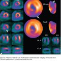
An example of four instantaneous BSPM distributions corresponding to activation/repolarization sequence initiated by epicardial pacing is shown in Fig. 12–3. Note that the color scale is adjusted to the instantaneous values of extrema; thus, spatial patterns of low-level potential distributions can be discerned as clearly as those with much higher potentials at the peak activation.
Figure 12–3.
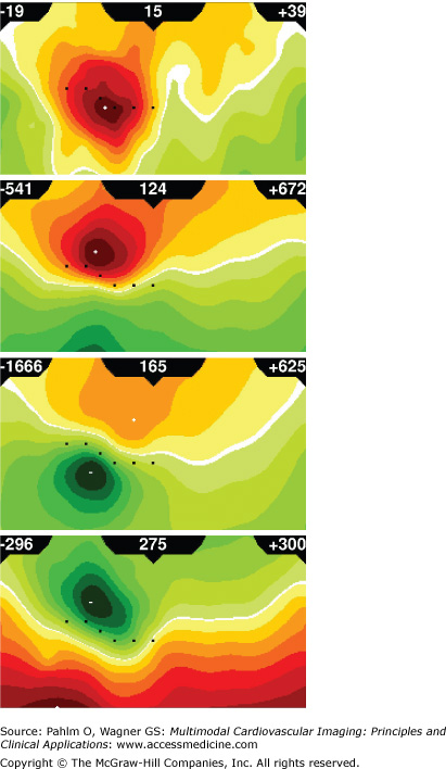
Body surface potential maps (BSPMs). Instantaneous BSPMs for epicardial pacing in the patient described in detail in the “Application of ECG Imaging in Clinical Electrophysiology” section are shown for the following time instants: 15 ms (early depolarization), 124 ms (advanced depolarization), 165 ms (peak depolarization), and 275 ms (early repolarization) after pacing at a basal inferior site. Each map is displayed on a cylindrical projection of the torso: the anterior chest projects on the left side of the map and posterior chest on the right side; left and right margins of each map correspond to the right mid-axillary line; top corresponds to the neck and bottom to the waist; and locations of six precordial leads of the conventional 12-lead electrocardiogram are shown as black squares. For color coding of potentials, yellow-to-red scale denotes positive potentials, and green scale denotes negative potentials. Regardless of amplitudes of extrema, there are always seven isopotential contours linearly distributed between zero and the larger of the two extrema (maximum/minimum). Amplitudes of maximum and minimum (in μV) are in the upper right and left corners, respectively, and time elapsed from the beginning of activation (in ms) is in the center of each panel.
We have shown previously15,16 that BSPM data acquired during catheter ablation of scar-related VT can assist with the identification of VT exit sites. Patients had BSPM data recorded during episodes of VT and endocardial pacing, and the data were analyzed to assess the similarity between the BSPM sequences occurring during VT and those induced by pacing. We found that, in general, the nearer the pacing site was to the exit site, the greater was the similarity between the VT and paced BSPM sequences. This suggested that BSPM can provide a useful adjunct to standard pace mapping. We realized, however, that additional processing—in particular, the inverse calculation of epicardial potentials/isochrones—would enhance the usefulness of the data gathered by BSPM. The rest of this chapter briefly reviews our methodology of inverse calculations and gives examples of their possible clinical use.
Forward and Inverse Problems of ECG
The forward problem of ECG involves computation of body surface potentials from specified cardiac generators that represent the electrical activity of the heart. The problem can be formulated in different ways, depending on the assumptions regarding the equivalent sources for the cardiac electrical activity and a representation of geometric and electrical properties of the volume conductor in which these sources are embedded.7,17,18
Numerical methods for solving the forward problem of ECG for arbitrarily shaped domain-wise homogeneous volume conductors have been in use since the 1960s; initially, the forward solution was performed to calculate potentials on the torso surface from dipolar sources.19-21 An alternative approach is to consider the distributed double-layer source on the epicardial surface as the equivalent generator.22 Barr et al7 introduced the mathematical formulation for computing linear transfer coefficients relating electric potentials on the epicardial surface and those on the body surface. This model—consisting of a homogeneous volume conductor bounded by realistically shaped surfaces of the heart and outer torso—was adopted in calculations presented in this chapter.
Let us consider the forward problem of ECG formulated as a calculation of the electric potentials ΦB = φ1B, … φmB at m area elements (or discrete points) on the body surface, SB, from the observed electric potentials ΦH = (φ1H, … φnH at n area elements (or discrete points) on the epicardial surface, SH. This leads to the boundary-value problem for Laplace equation in a homogeneous volume conductor that is bounded by smooth surfaces SB and SH.4,7 The final result, in matrix notation, is:
which expresses body surface potentials, ΦB, as a linear combination of epicardial potentials, ΦH, through the transfer matrix A. This forward relation is the basis for inverse-problem formulation in terms of epicardial potentials (see Equation 12–2).
Calculation of the transfer matrix A for Equation 12–1 requires a discretized representation of surfaces SB and SH of the torso model; this is accomplished by defining a set of points connected to form a three-dimensional mesh that represents each surface as a tessellation of planar triangles. Over the last decade, advanced imaging modalities—such as CT and MRI—have made it possible to acquire anatomic scans with high resolution, and thus, accurate patient-specific torso models can be readily generated.
We used axial CT scans (Siemens Sonata, Erlangen, Germany) acquired in supine position to generate patient-specific torso models. The location of body surface electrodes was estimated from known constraints: in-strip (5 cm) and between-strip (>2.5 cm) interelectrode distance, and correspondence with anatomic landmarks (location of precordial leads with reference to intercostal spaces). Figure 12–4 shows an example of the estimated distribution of 120 electrodes for BSPM on the patient-specific torso surface.
Figure 12–4.
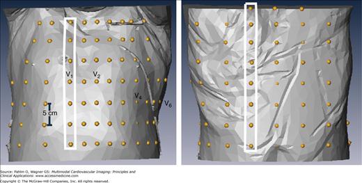
Dalhousie standard array of electrodes applied on the patient-specific torso surface. Anterior (left) and posterior (right) views of the torso surface with superimposed locations of 120 electrodes (yellow beads); there are 18 strips (as those in white rectangles) with four to eight electrodes in each, 12 strips on the anterior torso (extending from right to left mid-axillary line) and 6 strips on the posterior torso.
The 120 patient-specific locations of electrodes were then used as vertices to create a triangulated closed surface of the outer torso. A method was developed to make this patient-specific triangulation compatible with the Dalhousie standard 352-node torso geometry. (The Dalhousie standard torso consists of 352 nodes, which are vertices of 700 triangular area elements of the body surface.) Figure 12–5 illustrates the generation of the customized 352-node torso.
Figure 12–5.
Patient-specific modification of the standard Dalhousie torso. From left to right are anterior, left sagittal, and posterior views of the standard Dalhousie torso before scaling (blue) aligned with the triangulated surface (red) of patient-specific locations of the 120 surface electrodes (yellow beads). After scaling, node coordinates for the 352-node patient-specific torso model were generated by means of Laplacian interpolation of the patient-specific coordinates for electrode sites.
Generation of the discretized epicardial surface involved two steps: segmentation and triangulation. CT images were imported into the Amira package (Mercury Computer Systems, Chelmsford, MA), and an oblique slicing plane parallel to the coronary sinus was defined to facilitate segmentation of the ventricles down to the left ventricular apex. The labeled ventricles were then triangulated. Figure 12–6 shows the discretized epicardial surface, the section of the torso, and the oblique cut of the CT data through the coronary sinus to facilitate segmentation and discretization. Multiple passes of spatial filtering were applied to render a smooth surface.
Figure 12–6.
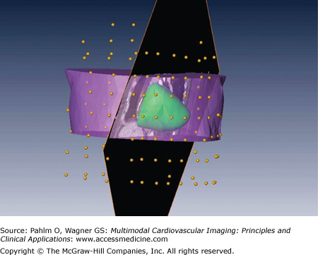
Segmentation and discretization of patient-specific epicardial surface. Anterior view of discretized epicardial surface (green), with selected sections of the torso (purple), oblique cut of the CT data through the coronary sinus (black), and locations of body-surface electrodes (yellow beads).
The objective of ECG imaging is to solve the inverse problem defined as the calculation of epicardial potential distributions from potential distributions acquired on the body surface (BSPM data). Whereas the mathematical solution of the forward problem of ECG is unique and depends continuously on the data (ie, the problem is “well posed”), the solution of the inverse problem may be neither unique nor depending continuously on the data (in which case, the problem is said to be “ill posed”), and small errors in the input data can generate unbound errors in the inverse solution. Thus, any attempted inverse solution usually requires that auxiliary constraints be imposed. The “ill-posedness” of the problem can be determined by examining the singular values of the transfer matrix A of Equation 12–1. Methods of mathematical regularization of ill-posed problems, most notably Tikhonov regularization,23 provide a key to their solution. Tikhonov regularization, applied to solving the inverse problem of ECG in terms of epicardial potentials, was our method of choice.
The inverse problem is to estimate in the Equation 12–1 epicardial potentials ΦH from the measured body-surface potentials ΦB and the transfer matrix A. Because both ΦB and ΦH are functions of time (body surface ECGs and heart surface electrograms, respectively), the inverse problem has to be solved at a series of time instants. At each instant, the solution for ΦH can be estimated by using Tikhonov regularization, which aims to solve a perturbed version of the least squares problem,
where ||.|| denotes the l2 norm, λ is the regularization parameter, and B is the regularizing operator. For a given A and appropriately selected λ > 0, a solution ΦH (λ) of the perturbed minimization problem in Equation 12–2 can be obtained from the generalized form of normal equations, which is derived by means of the generalized singular value decomposition.
Given a sequence of sampled BSPM data ΦB for a specific patient, together with the generalized singular value decomposition of the transfer matrix A and regularizing operator B for that patient (Appendix A), the solution for the epicardial potential distribution ΦH at each time step is calculated in two steps. First the regularization parameter λ is determined by one of several possible methods (Appendix B), and then, using Equation 12–A2 in Appendix A, the corresponding epicardial potential distribution ΦH is evaluated.
Application of ECG Imaging in Clinical Electrophysiology
The ECG inverse solution can be applied to aid catheter ablation of scar-related VT, which is still one of the most challenging procedures in clinical electrophysiology. The majority of these tachycardias are poorly tolerated or difficult to induce, and they frequently transform to other tachycardia morphologies.24 Successful ablation of scar-related VT requires an understanding of its mechanism and of the underlying electroanatomic substrate. Such insight can be partly achieved by percutaneous endocardial or epicardial mapping with a single catheter, which is steered to multiple sites to define the substrate for arrhythmia during sinus rhythm.25-27 However, this alone is often not sufficient for predicting successful ablation sites; some tachycardias are “unmappable” with point-by-point mapping, and alternative methods for identifying exit sites for these tachycardias have to be sought.28 One of the frequently used methods is pace mapping in the peri-infarct zone.29 Our objective here was to investigate how BSPM and the ECG inverse solution, in conjunction with pace mapping, can be used to facilitate radiofrequency ablation of scar-related VT.
Catheter mapping and ablation were revolutionized by electroanatomic mapping. The CARTO electroanatomic mapping system (Biosense Webster, Inc., Diamond Bar, CA) employed in this study uses a magnetic sensor in the catheter tip to detect its location in the magnetic field created by magnets placed beneath the patient, and a triangulated ventricular surface is displayed by a system (see Fig. 12–8), allowing visualization of various electrical measurements in real time.24,30 This system can be used to perform sinus rhythm voltage mapping, which involves sampling of the endocardial or epicardial bipolar electrograms recorded from an electrode catheter at multiple locations.25 Low-amplitude bipolar electrograms have been shown to correspond to infarcted myocardium, with amplitudes typically less than 0.5 mV over the dense scar.27 The CARTO system can also perform activation mapping, which annotates the anatomic construct with local activation times.25
The limitations of point-by-point mapping of activation sequences have led to the development of pace mapping methods for assessing the location of the mapping catheter relative to the reentry circuit.31-33 The procedure involves successive stimulation at various sites and comparing the paced QRS patterns with the template pattern of the clinical VT. Distinct patterns of BSPM distributions were observed for ectopic ventricular activation sequences initiated at various endocardial pacing sites for patients with idiopathic VT,34 as well as for patients who have had a prior myocardial infarction.33,35
Propagation of electrical activation in the diseased myocardium is discontinuous, and small differences in the pacing site can induce different propagation patterns and resulting QRS complexes.31,33 Nevertheless, the pacing from a catheter located near the exit of a reentry circuit of VT usually produces a QRS morphology similar to that of VT, with a short stimulus-to-QRS delay.36 Pacing that produces a QRS matching VT after a delay (stimulus-to-QRS interval >40 ms) has been shown to mark a site in a reentry channel within an infarct scar that is considered a good candidate for ablation.36 Trying to approach the exit site using sequential pace mapping can be challenging and requires an intuitive interpretation of the 12-lead ECG. We hypothesized that this process could be aided by BSPM and ECG imaging.
Some intraoperative studies involving endocardial and epicardial mapping have shown that scar-related VT does not always arise in the subendocardium.37-40 This evidence was further supported by studies using hearts explanted from patients who have had a myocardial infarction.41 VTs in which epicardial breakthrough preceded the earliest endocardial activity were reported,39 and some were successfully terminated by an epicardially directed procedure.38,42,43
Related posts:


Stay updated, free articles. Join our Telegram channel

Full access? Get Clinical Tree


