Fig. 1.
Electron energy loss spectrum (EELS) from DNA with zero-loss peak, plasmon peak, and superpositioned elemental edges which originate from excitation of inner-shell or core levels of phosphorus, carbon, nitrogen, and oxygen. The dashed line indicates the background extrapolation that is used to obtain the raw elemental signal (adapted from ref. 15).
One of the approaches for elemental mapping by EELS makes use of the energy filtering in the transmission electron microscope imaging mode (EFTEM) (3, 4). Electrons that are transmitted through a thin specimen enter the magnetic field of the spectrometer and are then dispersed according to their kinetic energy or velocity. A slit placed at the dispersion plane of the spectrometer’s magnetic prism selects electrons of a particular energy loss, which then travel through a series of lenses to form a high resolution image of the specimen on a two-dimensional array detector. By inserting an energy-selecting slit, elastically scattered as well as unscattered electrons are allowed to pass, which result in improvements in contrast in some applications.
To obtain element-specific maps from sectioned cells, it is typically necessary to record two images, one at an energy loss just above the atomic core level excitation threshold, with image intensity I post, and one at an energy loss just below the threshold, with image intensity I pre. By carefully subtracting a fraction of I pre intensity from I post intensity, it is possible not only to determine the net core edge signal but also to quantify the number of atoms of a particular element in the specimen using the theoretical scattering cross section for the core level excitation (2). The number of atoms n x of an element x in a pixel of dimension d can be determined from the net signal at energies above the core edge S x (Δ, β) measured in a band of width Δ defined by the energy-selecting slit and for a collection angle β, which is defined by the objective aperture:
![$$ {n}_{x}=\left[\frac{{S}_{x}(\Delta,b){d}^{2}}{{I}_{0}(\Delta,b)·{s}_{x}(\Delta,b)}\right],$$](/wp-content/uploads/2017/03/A213664_1_En_13_Chapter_Equ1.gif)
where I 0 (Δ, β) is the measured zero-loss intensity in the transmitted electron beam, for the same energy band and objective aperture, and σ x (Δ, β) is the inelastic scattering cross section for the core level excitation for the energy band Δ and collection semi-angle β (5). Usually the number of atoms of element x is much smaller than the total number of atoms in the volume of the specimen, so there is a strong background intensity underlying a relatively weak signal. Therefore, it becomes essential to subtract the background very carefully from the post-edge energy-selected image.
(1)
Several methods have been employed to take into account the background intensity (6, 7). The simplest approach is ratio mapping, for which post-edge I post is divided by the pre-edge intensity I pre. If the shape of the background remains constant across the entire image (which is rarely the case), the ratio value k x gives a simple representation of the distribution of element x:

(2)
However, it is useful to obtain a modified ratio, by subtracting a constant k 0 , which corresponds to the measured ratio value in a region of the specimen where the element x is known to be absent.
(3)
Multiplying this equation by I pre gives the so-called two-window intensity S x , which is an accurate measure of the core-edge signal, provided that the shape of the background remains constant over the field of interest.
(4)
When the specimen thickness is nonuniform, which often occurs, the shape of the spectral background varies significantly over the field of interest. Thus, the above mentioned method of calculating the core-edge signal becomes invalid. Previously, this change of spectral shape has been taken into account by collecting additional pre-edge images at different energy losses. For example, in the three-window method, two images are collected below the core-edge (8). By fitting the pre-edge background intensity as an inverse power function, its shape is allowed to vary across the image. However, for beam-sensitive biological specimens the electron dose is restricted and thus the three-window method drastically increases the statistical noise in the extrapolated background, which results in a substantial reduction in analytical sensitivity. For this reason, it is preferable to retain a two-window approach by modifying it to take into account subtle changes in the background shape as a function of the sample thickness t. In this case, it is convenient to measure the specimen thickness in units of inelastic mean free path λ, which can be readily determined from the fraction of transmitted electrons in the zero-loss peak:
(5)
Here, I unflt is the total unfiltered image intensity. The inelastic mean free path for plastic embedding material is typically 150–200 nm for a microscope accelerating voltage of 120 kV and 300–400 nm for a microscope operating at 300 kV.
To incorporate the thickness variation into the two-window method, we compute the spectral intensity as a function of t/λ using logarithmic Fourier deconvolution method (7). It is then possible to calculate the ratio k 0 as a function of t/λ, resulting in the k-curve or a fitted function, which provides a set of parameters that can be used to adjust the k-value at each imaged pixel. It is then straightforward to compute a thickness-corrected or modified two-window elemental map and write the following expression for the number of atoms in a pixel of dimension d.
![$$ {n}_{x}=\left[\frac{{I}_{\text{post}}(\Delta,b)-{k}_{0}\left(\frac{t}{l}\right){I}_{\text{pre}}(\Delta,b)}{{I}_{0}(\Delta,b)·{s}_{x}(\Delta,b)}\right]{d}^{2}.$$](/wp-content/uploads/2017/03/A213664_1_En_13_Chapter_Equ6.gif)
(6)
This ability to correct for thickness effects in elemental maps by using a t/λ dependent k-ratio enables two-window elemental mapping to be performed in specimens that are as thick as one inelastic mean free path, without artifacts due to plural inelastic scattering.
Here we will mainly discuss the application of the modified two-window method on mapping phosphorus (P) in sectioned cells in 2D as well as in 3D. Since DNA contains one phosphate group for every base in the structure, EFTEM imaging of phosphorus provides an intrinsic molecular label for nucleic acid, and can be combined with nitrogen imaging, which provides a means of distinguishing between DNA and protein complexes (see Fig. 2). It is not feasible to map the distribution of phosphorus in frozen hydrated cells, except at low spatial resolution, because of their high sensitivity to damage. EFTEM can be used to image phosphorus in cells or tissues that have been prepared by high pressure freezing and freeze substitution or conventional chemical fixation, embedding and sectioning. In such preparations, it is important to avoid heavy metal fixatives and stains that could interfere with the phosphorus edge in the energy loss spectrum. Until recently EFTEM phosphorus mapping of cells in unstained plastic sections has involved the collection of two-dimensional maps. By combining EFTEM with tomography, it is now possible to obtain three-dimensional phosphorus distributions of cellular components (9).
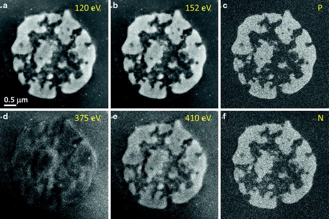
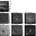
Fig. 2.
EFTEM elemental mapping of a thymocyte nucleus. (a) and (b) show the P L2,3 pre-edge image at 120 eV and post-edge image at 152 eV, which are used to calculate the 2D phosphorus map shown in (c). (d) and (e) are the N pre-edge image at 375 eV and N post-edge image at 410 eV, which are used to calculate the 2D nitrogen map shown in (f). Major components of the thymocyte nucleus are densely packed DNA containing phosphorus and nitrogen, and protein containing nitrogen but negligible phosphorus. Nitrogen concentrations attributed to protein structures are visible in regions that contain low levels of chromatin regions that appear dark in the phosphorus map (15).
2 Materials
For performing EFTEM imaging and for processing the acquired data, the following equipment is recommended, with the manufacturer listed. These are suggestions only, since different manufacturers are available for each item:
2.1 General Supplies
1.
Acetone.
2.
Glutaraldehyde.
3.
Epon-Aradite (Ted Pella): EMbed-812 and Araldite-502.
4.
10 nm colloidal gold (SPI Inc.).
5.
400 Mesh bare Copper Finder grids (Electron Microscopy Sciences, USA).
2.2 Instrumentation
1.
Glow discharger.
2.
High Pressure Freezer (HPM10, Bal-Tec, Switzerland).
3.
Freeze-substitution system (EM-AFS, Leica Microsystems, Germany).
4.
Ultramicrotome (EM UC6, Leica Bannockburn, IL).
5.
Carbon evaporator (Auto 306, BOC Edwards, UK).
6.
Non-tilt and tomography holder (Fischione Instruments, USA).
7.
100–300 kV transmission electron microscope (Tecnai TF30, FEI company, The Netherlands).
8.
Tridiem post-column imaging filter (Gatan, USA).
9.
2k × 2k Ultrascan cooled CCD detector for direct digital recording (Gatan, USA).
Items 2 and 3 are required only if preparing samples by high-pressure freezing (Subheading 3.1.1).
2.3 Software
1.
Digital Micrograph (DM) tomography software for automatic data acquisition (Gatan, USA).
2.
Filter Control software (Gatan, USA).
3.
IMOD software for alignment and reconstruction of tomographic tilt series (http://bio3d.colorado.edu/imod/ University of Colorado at Boulder, USA) (10).
3 Methods
Here we describe the steps taken for specimen preparation, general microscope setup, data acquisition and processing obtained using several imaging modes that generate quantitative elemental maps.
3.1 Specimen Preparation
To obtain resin-embedded, unstained sectioned cells (see Note 1) for elemental mapping in EFTEM imaging mode, the following is a brief description of the specimen preparation:
3.1.1 High Pressure Freezing
1.
Specimens are transferred to sample carriers, for example Drosophila larvae/Caenorhabditis elegans in 15% sucrose.
2.
The samples are then frozen in a high pressure freezer and freeze-substituted in acetone containing 0.2% glutaraldehyde at −90°C for 3 days and then slowly warmed (5°C/h) to 20°C.
3.
After rinsing several times in acetone, the samples are infiltrated with Epon-Aradite and polymerized at 60°C for 2 days (see Note 2).
4.
The sections are cut to a thickness of 90–150 nm (see Note 3), and picked up on 400 mesh bare copper grid.
5.
To ensure the stability of the sections under the electron beam, 5–10 nm carbon films are evaporated directly onto the copper grids containing the specimens using a carbon rod mounted in the evaporator.
6.
The grids are glow-discharged in air for 30 s and 10 nm colloidal gold is deposited on top and bottom of the grids (see Note 4). After 5 min, the samples are thoroughly washed with de-ionized water to remove excess reagents.
3.1.2 Chemical Fixing
1.
Samples are post-fixed with 2.0% glutaraldehyde in PBS. For example wild-type mouse thymocytes are post-fixed for 5 min.
2.
After extensive washing in PBS, the specimens are dehydrated in ethanol solutions of 30, 50, 70, 90% for 10 min and 100% for 45 min, before being infiltrated with Epon-Araldite: 30% Epon-Araldite and ethanol for 2 h, 50% Epon-Araldite and ethanol for 4 h, 75% Epon-Araldite for 12 h and 100% for 1 day.
3.
The embedded blocks are then polymerized at 60°C for 2 days.
4.
The sections are cut to a thickness of 90–150 nm, and picked up on 400 mesh bare copper finder grids.
5.
The rest of the steps are the same as mentioned above, for the high-pressure frozen preparation.
3.2 General Microscope Setup in EFTEM Imaging Mode
Low noise image acquisition is an important step to ensure generation of nanoscale quantitative elemental maps, whether it is in two or three dimensions. Listed below are the steps needed for data acquisition in the EFTEM imaging mode of the electron microscope:
3.2.1 D EFTEM Imaging
1.
 Introduction: Nanoimaging Techniques in Biology
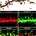 Two-Color STED Imaging of Synapses in Living Brain Slices
 Secondary Ion Mass Spectrometry Imaging of Biological Membranes at High Spatial Resolution
 High Data Output Method for 3-D Correlative Light-Electron Microscopy Using Ultrathin Cryosections
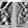 Functional AFM Imaging of Cellular Membranes Using Functionalized Tips
 Single-Molecule Tracking of mRNA in Living Cells


Load the alignment file in the microscope software as well as in Filter Control, which has previously been aligned in the EFTEM mode.
Related posts:
Introduction: Nanoimaging Techniques in Biology
Two-Color STED Imaging of Synapses in Living Brain Slices
Secondary Ion Mass Spectrometry Imaging of Biological Membranes at High Spatial Resolution
High Data Output Method for 3-D Correlative Light-Electron Microscopy Using Ultrathin Cryosections
Functional AFM Imaging of Cellular Membranes Using Functionalized Tips
Single-Molecule Tracking of mRNA in Living Cells
Stay updated, free articles. Join our Telegram channel
Full access? Get Clinical Tree
