(1)
Amersham, Buckinghamshire, UK
Abstract
This chapter provides the elements of quantum scattering theory which shall be used throughout this book. The general scattering problem is reviewed in the context of scattering and time evolution operators and recognises that the observables are the pre- and post-scattering asymptotic states. Quantum perturbation theory is developed with the two linked goals of deriving an expression for the transition probability rate between two quantum states (Fermi’s Golden Rule) and the scattering amplitude and differential cross section (first Born approximation). The Born approximation is derived through the Lippmann–Schwinger equation. The chapter concludes with a phase shift analysis of the scattering problem.
2.1 Introduction
The topic of this book is that of the interactions of a moving charged particle as it slows down within a medium which result in kinetic energy loss through energy transfers to the medium. These interactions are referred to as ‘scatters’ or ‘collisions’1 as the projectile will be scattered from its original trajectory into a different direction, a process which may or may not involve a significant transfer of energy from the projectile to the target. A light projectile, such as an electron, scattered from a heavy nucleus will not, due to the requirement of the simultaneous conservations of energy and momentum, impart significant recoil energy to the nucleus, and little energy is transferred to the medium containing that nucleus. On the other hand, if the projectile and target have masses which are comparable or of the same order of magnitude (e.g. as in electron–electron scatter or the scatter of an α-particle from a light nucleus), then significant energy transfer can occur (see Appendix D). These interactions are probabilistic in nature and are described by differential cross sections. On the other hand, the kinematics of the scatter is not probabilistic and is well defined. For radiation dosimetry calculations, we are most interested in the probabilities of given amounts of kinetic energy being transferred through a scatter. This chapter provides the basic components of the quantum ‘toolkit’ required to calculate these interactions and their consequences. It does not intend to be a full and detailed exposition of quantum scattering theory: it is expected that the reader will already be at least aware of much of the material summarised here, and that, in a sense, this chapter provides a review of those aspects relevant to the calculation of the transfer of the kinetic energy of a moving charged particle to the medium it transverses. More specific attributes of the theory that we make singular or infrequent use of will be introduced at the time of the relevant discussion elsewhere in this book. The reader who wishes further detailed description of quantum scattering theory may refer to the texts cited in the references to this chapter.
Depending upon the physics application, there can be a variety of definitions of ‘elastic’ and ‘inelastic’ scatter. In this book, an elastic scatter is defined as one in which the total kinetic energy is conserved: the sum of the kinetic energies of the projectile and target in the initial state is equal to the sum of the kinetic energies of the products in motion in the final state. On the other hand, an inelastic scatter is defined as one in which the sum of the post-scatter kinetic energies is less than that of the pre-scatter state. This would be due to the diversion of the initial state kinetic energies to internal degrees of freedom provided by the scattering system. Such channels would include atomic or nuclear excitation and ionisation.2 In general, we will consider the interaction to be that of the scattering from the Coulomb potential energy of  , where z and Z are the electric charges of the projectile and target in integer multiples of the fundamental electric charge, e, or a Yukawa-type modification of the Coulomb potential as a model of electrostatic screening. Should the scattering centre not be well modelled as infinite mass or itself be in motion, then the scattering problem can be solved in the centre-of-mass system in which the projectile mass in the calculation is replaced by the reduced mass of the projectile and target and the target considered to be a potential. Even the inelastic scatter from an atomic electron which is ejected as a consequence can be well approximated as an elastic interaction if the kinetic energies involved greatly exceed the electron binding energy. Indeed, it will often be the case that the atomic electron can be considered to be at rest if the projectile velocity greatly exceeds the orbital velocity of the electron.3
, where z and Z are the electric charges of the projectile and target in integer multiples of the fundamental electric charge, e, or a Yukawa-type modification of the Coulomb potential as a model of electrostatic screening. Should the scattering centre not be well modelled as infinite mass or itself be in motion, then the scattering problem can be solved in the centre-of-mass system in which the projectile mass in the calculation is replaced by the reduced mass of the projectile and target and the target considered to be a potential. Even the inelastic scatter from an atomic electron which is ejected as a consequence can be well approximated as an elastic interaction if the kinetic energies involved greatly exceed the electron binding energy. Indeed, it will often be the case that the atomic electron can be considered to be at rest if the projectile velocity greatly exceeds the orbital velocity of the electron.3 Our study of scatter, however, will not consider the pure multi-body state.4 There is no need to introduce this complication as the flux of projectiles and the density of targets are such that, at the microscopic level, a binary interaction need only be considered.5 Hence, we will restrict ourselves to the problems of a single projectile incident to a single target or potential. As the scattering problem is fundamental to many diverse fields of physics in addition to our interest in radiation dosimetry, we will model our derivations of the calculated tools provided by this chapter upon the most general aspects of particle scattering.
2.2 The General Scattering Problem
2.2.1 Initial and Final Observable States
The general scattering problem must be thought of as follows. Before and after the interaction in those regions of space where the scattering potential can be assumed to be effectively equal to zero, the particles are considered to be described by wave packets which are solutions to the homogeneous Schrödinger equation. The Heisenberg uncertainty principle  states that one cannot precisely measure the position of the particle without a corresponding uncertainty in determining its momentum. In this region of space, the Hamiltonian is the free representation, H 0, with the eigenvalue of the particle’s kinetic energy, E. This implicitly requires the static potential U which resulted in the scattering of the potential to be non-zero only within a finite range a. More precise definitions of this requirement include, first, that the potential be locally square integrable
and, second, that the magnitude of the potential be limited at infinite distances,
states that one cannot precisely measure the position of the particle without a corresponding uncertainty in determining its momentum. In this region of space, the Hamiltonian is the free representation, H 0, with the eigenvalue of the particle’s kinetic energy, E. This implicitly requires the static potential U which resulted in the scattering of the potential to be non-zero only within a finite range a. More precise definitions of this requirement include, first, that the potential be locally square integrable(2.1)
(2.2)
Within the range a of the potential, the total Hamiltonian which includes the potential  must be considered as to be discussed. Note that we have used the general form of the potential as having a directional dependence through the use of the vector
  as the argument rather than the scalar quantity,
  . While a well-known potential having a directional dependence is that of the tensor nuclear force associated with the deuteron, such potentials are of no interest to the scattering problems examined in this book, although the initial steps of derivations will use
  for generality before adopting
  when it becomes appropriate. The potentials that we will consider (the attractive/barrier well, the Yukawa and the Coulomb) are all central. However, in particular, it should be noted that the
  nature of the Coulomb potential means that that potential cannot meet the conditions of either (2.1) or (2.2). This necessitates either the careful use of perturbation theory for the Yukawa potential
  where, following integration, the screening parameter κ is set to zero or else a full and precise calculation of the Coulomb scattering problem is performed, as shall be shown in Chap. 4.
must be considered as to be discussed. Note that we have used the general form of the potential as having a directional dependence through the use of the vector as the argument rather than the scalar quantity, . While a well-known potential having a directional dependence is that of the tensor nuclear force associated with the deuteron, such potentials are of no interest to the scattering problems examined in this book, although the initial steps of derivations will use for generality before adopting when it becomes appropriate. The potentials that we will consider (the attractive/barrier well, the Yukawa and the Coulomb) are all central. However, in particular, it should be noted that the nature of the Coulomb potential means that that potential cannot meet the conditions of either (2.1) or (2.2). This necessitates either the careful use of perturbation theory for the Yukawa potential where, following integration, the screening parameter κ is set to zero or else a full and precise calculation of the Coulomb scattering problem is performed, as shall be shown in Chap. 4.Continuing from these requirements, let us next consider the macroscopic fundamentals of particle scattering from the perspective of the experimentalist who can observe only the macroscopic initial state and the macroscopic consequences of the scatter. It is from these observations that the microscopic details of the scattering process (e.g. the form of the scattering potential) are deduced. The experimentalist must first create or determine a well-defined initial state consisting of a projectile incident to a target. Having done so, he will then detect and measure the final state achieved as a consequence of the scatter. In practical medical applications, the initial state can be that of a flux of charged particles external to the body directed towards tissue. This flux may be generated by an accelerator (e.g. a linear accelerator or a cyclotron) in which charged particles are set into motion, filtered through a momentum analyser and then collimated to form a beam which is, macroscopically, well defined in terms of momentum and spatial distribution. This is also the result of the external beam being of x- or γ-rays which produces a secondary charged particle flux within the medium through Compton scatter, photoelectric absorption or, if highly energetic, photonuclear reactions. The energy spectra of these charged particles will be defined by the combination of the photon energy spectrum and the kinematics of the physics of these photon–matter interactions. Another scenario arises from neutron irradiation in which a secondary charged particle flux arises from neutron–proton elastic scatter. Charged particle fluxes can also be generated by the nuclear decays of a distributed source of a radionuclide within tissue resulting in the emission of α-particles, electrons or positrons. In this case, the kinetic energies of the charged particles are dictated by the kinematics of the nuclear decay and are generally constrained to a spectrum.6 Further, the emission of these charged particles will be isotropic with respect to the site of emission. A photon-emitting internally distributed radionuclide also generates secondary electrons in the same manner as an external beam of photons.7 In all cases, the initial state can be defined by the experimentalist through measurement or calculation who, after the scattering, will detect the scattered particle with an apparatus.8 Depending upon the application, this apparatus could provide information on, for example, the momentum, scatter direction and spin orientation of the scattered particle and/or of the recoiling target. Hence, to repeat, the experimentalist will know only the initial state of the projectile and its final state following the interaction, at distances far from the scattering centre and at a time which may be treated as being infinite in comparison to the actual duration of the scattering interaction linking the initial and final observed states. In other words, the experimentalist has information on the asymptotic forms of the initial and final states only. Clearly, what is of interest is the determination of the probability that the known initial state will yield the observed final state. This leads to the question of, what is the nature of the interaction that bridged the initial and final states? Of more practical and immediate interest to our application of this theory to the dosimetry problem is the question of, what is the probability of a given final state, following the transfer of energy to the medium, occurring for a given initial state?
To place the above into a more quantitative representation, the initial observed state is characterised by the wavefunction  and that of the final observed state is by a wavefunction
  with both states existing far from the scattering centre and, thus, being solutions to the homogeneous Schrödinger equation. An example of this is provided by the geometry of Fig. 2.1 in which
  is incident to the potential centred at the origin,
  . Following the interaction with this potential, the particle is deflected from its original trajectory and is described asymptotically by the wavefunction
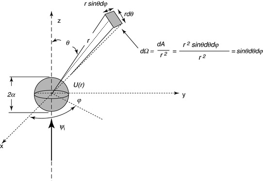
  . This deflection may or may not be accompanied by the loss of energy from the projectile and its transfer to the scattering centre. In this problem, we wish to determine the probability of the particle being scattered through the angle θ into the differential solid angle element dΩ at a distance r from the scattering centre. Note that for a central and isotropic potential
  , there is no dependence upon the azimuthal scattering angle, φ. In many practical cases in dosimetry calculations, we are not interested directly in the directional changes caused by the scatter but, rather, the changes in energy (i.e. energy loss) that occur as a result. This is often obtained by first calculating the directional dependence of the scatter and then incorporating the kinematics of two-body scatter.
and that of the final observed state is by a wavefunction with both states existing far from the scattering centre and, thus, being solutions to the homogeneous Schrödinger equation. An example of this is provided by the geometry of Fig. 2.1 in which is incident to the potential centred at the origin, . Following the interaction with this potential, the particle is deflected from its original trajectory and is described asymptotically by the wavefunction . This deflection may or may not be accompanied by the loss of energy from the projectile and its transfer to the scattering centre. In this problem, we wish to determine the probability of the particle being scattered through the angle θ into the differential solid angle element dΩ at a distance r from the scattering centre. Note that for a central and isotropic potential , there is no dependence upon the azimuthal scattering angle, φ. In many practical cases in dosimetry calculations, we are not interested directly in the directional changes caused by the scatter but, rather, the changes in energy (i.e. energy loss) that occur as a result. This is often obtained by first calculating the directional dependence of the scatter and then incorporating the kinematics of two-body scatter.Fig. 2.1
Scattering geometry. The wavefunction is incident along the z-axis to a central and isotropic potential, U(r), with an effective range a centred at the origin. The wave is scattered to yield a quasi-spherical outgoing wave representing the probability of the scattered particle being at a certain point in space, a fraction of which traverses the differential solid angle element, dΩ, at a distance r from the scattering centre
With the exception of the influence of the Coulomb potential (which has infinite range), outside the range a of the potential, the particles are in free motion and are not influenced by the potential that gave rise to the scattering. Further, as the time of the actual interaction is very short (of the orders of 10−15 to 10−12 s or less), we can consider the incident and final states to be those of the distant past and remote future,  . That is, at these limits of time, there are no interactions between the projectile and the scattering force, and the scattering potential does not affect the projectile. These free and final states are described, in state vector form, by the time-dependent Schrödinger equation:
When the particle is within the range of the potential  and is under its influence, the total Hamiltonian is the sum of the free Hamiltonian and the perturbing potential:

with the corresponding time-dependent Schrödinger equation
for the total state wavefunction, ψ(t). The asymptotic requirement of the scattering problem is that, as  , the total wavefunction described by (2.5) asymptotically approaches the unperturbed wavefunctions,
  and
and  . We now examine operators that describe the scattering process and which lead to the physical observables seen by the experimentalist. The relevant operator algebra is summarised in Appendix C.8.
. That is, at these limits of time, there are no interactions between the projectile and the scattering force, and the scattering potential does not affect the projectile. These free and final states are described, in state vector form, by the time-dependent Schrödinger equation:(2.3)
and is under its influence, the total Hamiltonian is the sum of the free Hamiltonian and the perturbing potential:(2.4)
(2.5)
, the total wavefunction described by (2.5) asymptotically approaches the unperturbed wavefunctions, and . We now examine operators that describe the scattering process and which lead to the physical observables seen by the experimentalist. The relevant operator algebra is summarised in Appendix C.8.2.2.2 Scattering and Time Evolution Operators
As the experimentalist can only measure the initial and final states, any information regarding the interaction must be determined indirectly through comparison of these two states, one occurring at an earlier time (pre-scatter) and the other at a later time (post-scatter). Hence, what needs to be understood by the theorist (i.e. us, who are calculating the radiation dosimetry resulting from such an interaction) is the descriptor of the scattering process in which the quantum mechanical operator S links these initial and final states of the projectile:
(2.6)
As the experimentalist can extract only the physical observables associated with the wavefunctions  and
and  , such as the fraction of the incident particle flux scattered into a solid angle set about a given direction, it will be the scattering operator that contains all of the information that links the two systems of the initial and final states and which must be determined from these experimental observables.
and , such as the fraction of the incident particle flux scattered into a solid angle set about a given direction, it will be the scattering operator that contains all of the information that links the two systems of the initial and final states and which must be determined from these experimental observables.Upon inspection, this scattering operator must have two fundamental properties. First, it must be unitary:
(2.7)
This property means that the sum of the probabilities of all of the final states that can possibly arise from a given initial state must equal unity. It follows from (2.7) that the adjoint of S must equal the inverse of S:

(2.8)
The third property of the scattering operator is that it must be stationary (i.e. it has no time dependence).
The S-matrix elements provide the physical observables presented to the experimentalist. That is, by using the Dirac bra–ket notation (described in Appendix E), the squared modulus  is proportional to differential cross sections which describe the measurable probabilities of the transition from the initial state
  to the final state
  occurring. In general, the state variables affected by charged particle scattering that are of interest are usually energy or momentum, scattering direction and intrinsic spin. The effect of scattering upon the energy variable is clearly of the greatest interest in a dosimetry calculation. This requires the integration of the scattering cross section over all scattering angles as the directions of the particles in the post-scattering state are generally of no interest in a dosimetry calculation, except for the case of regions in the vicinity of an interface between two radiologically differing media. Further, should it be necessary to account explicitly for the effects of intrinsic spin, this is done by first recognising that the pre- and post-scatter spin orientations are not known nor are of interest in medical radiation applications. In this case, the incident beam of particles and the targets are unpolarised, and so every possible state of spin orientation has the same a priori probability of existing. Hence, one first averages the calculation over the initial spin states as the contributions of the initial spin states are incoherent. One then sums over the final spin states. We will return to this specific problem, for example, in our derivation of the Mott scatter differential cross section for a Dirac spin-½ projectile, such as the electron.
is proportional to differential cross sections which describe the measurable probabilities of the transition from the initial state to the final state occurring. In general, the state variables affected by charged particle scattering that are of interest are usually energy or momentum, scattering direction and intrinsic spin. The effect of scattering upon the energy variable is clearly of the greatest interest in a dosimetry calculation. This requires the integration of the scattering cross section over all scattering angles as the directions of the particles in the post-scattering state are generally of no interest in a dosimetry calculation, except for the case of regions in the vicinity of an interface between two radiologically differing media. Further, should it be necessary to account explicitly for the effects of intrinsic spin, this is done by first recognising that the pre- and post-scatter spin orientations are not known nor are of interest in medical radiation applications. In this case, the incident beam of particles and the targets are unpolarised, and so every possible state of spin orientation has the same a priori probability of existing. Hence, one first averages the calculation over the initial spin states as the contributions of the initial spin states are incoherent. One then sums over the final spin states. We will return to this specific problem, for example, in our derivation of the Mott scatter differential cross section for a Dirac spin-½ projectile, such as the electron.The time-dependent Schrödinger equation of (2.5) yields a determinism in that by knowing the state of the system described by the wavefunction  at a prior time
  , the state will be known for all time. In other words, solving the scattering problem is to solve the time evolution of the quantum system (or the two subsystems of incident and scattered particles in the case of scattering). For example, this time evolution can be described by
where  is the time evolution operator and which clearly must be linear. It follows from (2.9) that the inverse operator
  must also exist due to time invariance. Substituting (2.9) into the time-dependent Schrödinger equation of (2.5) yields the result
at a prior time , the state will be known for all time. In other words, solving the scattering problem is to solve the time evolution of the quantum system (or the two subsystems of incident and scattered particles in the case of scattering). For example, this time evolution can be described by(2.9)
is the time evolution operator and which clearly must be linear. It follows from (2.9) that the inverse operator must also exist due to time invariance. Substituting (2.9) into the time-dependent Schrödinger equation of (2.5) yields the result(2.10)
The solution to the differential equation of (2.10) yields an expression for the time evolution operator  :
:
:(2.11)
Further properties of the operator follow from the above equations. Clearly,  follows from (2.11), as expected. Also, as the conservation of probability demands that the scalar product of the wavefunction at different times must remain constant (as demonstrated below), or
then the insertion of (2.9) into (2.12) gives
which subsequently demonstrates the unitarity of the time evolution operator:
follows from (2.11), as expected. Also, as the conservation of probability demands that the scalar product of the wavefunction at different times must remain constant (as demonstrated below), or(2.12)
(2.13)
(2.14)
For example, as the inverse of the time evolution operator  exists, then
which follows from the conservation of probability. In order to ensure the above,  must remain independent of time which requires that the Hamiltonian be Hermitian (i.e. H † = H). To assure ourselves that this condition is met, let us consider the complex conjugate (adjoint) of the Schrödinger equation:
which we then multiply by  to give
exists, then(2.15)
must remain independent of time which requires that the Hamiltonian be Hermitian (i.e. H † = H). To assure ourselves that this condition is met, let us consider the complex conjugate (adjoint) of the Schrödinger equation:(2.16)
to give(2.17)
Subtracting this result from its complex conjugate results in
(2.18)
2.3 Presentation of Calculation Tools
In the remainder of this chapter, we present the tools for calculating the physical observables associated with the scattering of a charged particle. In nearly all cases, the chapter will be restricted to nonrelativistic theory. The rationale for this is that in medical applications, the relativistic theory for a Dirac spin-½ particle is only applicable to fast electrons and positrons under the influence of the Coulomb potential. This discussion is deferred to Chap. 4 where the discussions of relativistic quantum scattering theory are presented in the context of Mott scatter and to Chaps. 8 and 9 for the topics of the Bethe, Møller, Bhabha and Bloch theories.
2.4 Quantum Perturbation Theory
2.4.1 Fermi’s Golden Rule
As noted earlier, the scattering of a particle can be described by the transition from the initial state denoted by the incident particle’s kinetic energy E and three-vector momentum p to a final state of kinetic energy  and momentum
  . The inclusion of intrinsic spin as an additional variable to be considered in the scatter is discussed in later chapters in relation to electrons and positrons and is not considered here. The probability of a transition occurring between two quantum states can be described through time-dependent perturbation theory. Its most practical appearance is that of Fermi’s Golden Rule which we will make substantial use of and will derive in this section.
and momentum . The inclusion of intrinsic spin as an additional variable to be considered in the scatter is discussed in later chapters in relation to electrons and positrons and is not considered here. The probability of a transition occurring between two quantum states can be described through time-dependent perturbation theory. Its most practical appearance is that of Fermi’s Golden Rule which we will make substantial use of and will derive in this section.We begin the derivation by considering a quantum system in steady state and described by the free Hamiltonian H 0. As noted before, this Hamiltonian describes the scattering system in which the projectile, either before or after scattering, is outside of the range of the influence of the perturbing potential. Schrödinger’s equation for this particular state is
(2.20)
A solution to this equation can be written in terms of a series of eigenstates which accounts for the evolution of the system over time:
where the coefficients a k,0 are constants. We next consider the case when this system is perturbed by a time-dependent potential, U(t), and attempt to determine the probability of a particular final state being achieved through a transition from the initial state. This state during the perturbation reflects the brief time of the actual scatter when the particle is under the influence of the scattering potential. We begin the calculation by writing the total Hamiltonian of the interacting system as
(2.21)
(2.22)
A dimensionless weighting parameter, λ, has been included to scale the influence of the potential for the purpose of enabling a perturbative calculation. The Schrödinger equation of this perturbed system is
(2.23)
As the eigenstates ψ k must form a complete set, we can write the wavefunction of the perturbed state as
where the coefficients, unlike those of (2.21), have a time dependence due to the potential. These coefficients are such that we define them at time t = 0 as  , and we interpret the squared modulus
  as representing the probability of finding the perturbed system in the k-th state at the time t. These time-dependent coefficients are determined by substituting this series representation of the wavefunction into the Schrödinger equation:
![$$ \begin{array}{clclclclc}{ i\hbar \left[ {\sum\limits_k {\left( {\frac{{\mathrm{ d}{a_k}(t)}}{{\mathrm{ d}t}}{\psi_k}{e^{{-i\frac{{{E_k}t}}{\hbar }}}}-i\frac{{{E_k}}}{\hbar }{a_k}(t){\psi_k}{e^{{-i\frac{{{E_k}t}}{\hbar }}}}} \right)} } \right] \hfill =\left( {{H_0}+ U(t)} \right)\sum\limits_k {{a_k}(t){\psi_k}{e^{{^{{-i\frac{{{E_k}t}}{\hbar }}}}}}}.}\end{array} $$](/wp-content/uploads/2016/04/A306762_1_En_2_Chapter_Equ000225.gif)
(2.24)
, and we interpret the squared modulus as representing the probability of finding the perturbed system in the k-th state at the time t. These time-dependent coefficients are determined by substituting this series representation of the wavefunction into the Schrödinger equation:(2.25)
Separating the free Hamiltonian and perturbative terms in (2.25) leads to the two equalities:
(2.26)
(2.27)
The result given by (2.26) is trivial and is ignored. The effect of the perturbative potential alone upon the system is described by (2.27). By using the Dirac bra–ket formalism, (2.27) is rewritten as
(2.28)
We next multiply both sides of (2.28) by the bra  of the final state (i.e. that following the perturbation) and integrate the wavefunctions over all space:
of the final state (i.e. that following the perturbation) and integrate the wavefunctions over all space:(2.29)
From the definition of the scalar product and using the orthonormality of states (which follows from the definition of the scalar product),  , where δ mn is the Kronecker δ-function, (2.29) becomes
where the matrix element relating the final state f to the state k is defined as  . Rearranging (2.30) gives the derivatives of the coefficients as a series:
where we have defined the frequency of the transition from the kth state to the final f state as
, where δ mn is the Kronecker δ-function, (2.29) becomes(2.30)
. Rearranging (2.30) gives the derivatives of the coefficients as a series:(2.31)
(2.32)
It is now that we make use the coefficient λ that weights the influence of the perturbative potential. We demand that the strength of the potential relative to the eigenvalues of the steady-state Hamiltonian be weak. Consequently, the coefficients a k (t) are then expanded through a power series of the coefficient λ:
(2.33)
Then, by equating the coefficients of equal powers of λ, we obtain the following expressions for the derivatives of the coefficients:

and
(2.35)
(2.36)
In order to use these results to calculate the coefficients, let us assume that the perturbing potential is ‘switched on’ at time  and remains constant for
and remains constant for (2.37)
 is Heaviside’s function defined here as
(2.38)
In this model, we further assume that the system is initially in a single and well-defined state  for
for  . Thus,
  and the remaining coefficients at time t are then found by integrating (2.36) where, as
  has been previously defined as being small, the calculation need only be limited to
where  . The probability that a transition from the state
  to the state
  occurring at time t is
for . Thus, and the remaining coefficients at time t are then found by integrating (2.36) where, as has been previously defined as being small, the calculation need only be limited to(2.39)
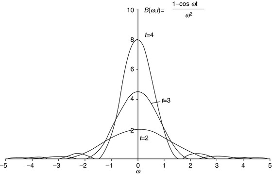
. The probability that a transition from the state to the state occurring at time t is(2.40)
As shown in Fig. 2.2, the function B(ω,t) is at a maximum for ω = 0, and the sharpness of this maximum increases with increasing t. This observation demonstrates that the probability of a given transition occurring between two states is greater when the energy difference between the initial and final states is smaller.
However, in reality, in a quantum transition, it is unlikely that the final state will have a singular energy associated with it. The most likely case will be, in fact, that of an ensemble of neighbouring states centred around  with different (energy) eigenvalues around the final-state energy, E f . As a consequence, the transition probability must then be integrated over this ensemble of energy eigenvalues:


with different (energy) eigenvalues around the final-state energy, E f . As a consequence, the transition probability must then be integrated over this ensemble of energy eigenvalues:(2.41)
Related posts:
Stay updated, free articles. Join our Telegram channel
Full access? Get Clinical Tree
