Estimation of Microscopic Anisotropy in Macroscopically Isotropic Substrates Using Diffusion MRI

(1)

where $S_\parallel$ is the signal for the dPFG sequence with parallel gradients, $S_\perp$ is the signal for the dPFG sequence with perpendicular gradients, $q = \gamma G \delta$ is the wavenumber, $\gamma$ the gyromagnetic ratio, G the gradient strength, $\delta$ the pulse duration and $\epsilon$ depends on pore size and eccentricity. For spherical pores $\epsilon = 0$ . To normalize $\epsilon$ with respect to size, [12] introduced the fractional eccentricity index FE which varies between 0 (isotropic pores) and 1 (elongated pores):

$\begin{aligned} FE = \sqrt{\frac{\epsilon }{\epsilon + 3 \varDelta ^2 ADC^2 /5}} \end{aligned}$

(2)

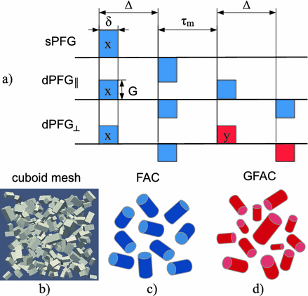
where $\varDelta$ is the diffusion time (see Fig. 1) and ADC is the apparent diffusion coefficient which reflects the length scale of the substrate.

3 Methods

This section presents the simulations and models we use in this paper to illustrate the feasibility of estimating pore shape and size distribution from diffusion MRI data using a model-based approach.

3.1 Data Synthesis

To synthesize diffusion data we use the MC simulator in Camino [18] with a mesh-based substrate. The mesh consists of 200 randomly oriented cuboids with two equal sides ( $$l_x = l_y$$

) and a gamma distribution of sizes, as illustrated in Fig. 1b. We choose a different geometric model to synthesize the data in order to emphasize the robustness of our approach when the geometry is not a perfect match. We prefer cuboids over ellipsoids due to the reduced computational complexity of the mesh. The parameters of the model are the mean width of the cuboid $$l_x$$

, the ratio between the height and width $$E = l_z/l_x$$

(eccentricity), which is the same for all sizes, the gamma distribution shape parameter a and the diffusivity constant D. We construct separate substrates for each combination the following parameter values: $l_x = \{2, 4, ..., 12\}\,\varvec{\mu }$ m, $E = \{1,1.5,2,2.5,3\}$ , $a = \{2.5,10,\infty \}$ ( $a\rightarrow \infty$ yields identical pores) and $$D = 2E-9$$

s/m

. The MC simulation has 1000 time steps and 20000 walkers, all located inside the pores. Noise, with a Rician distribution and a signal-to-noise ratio (SNR) of 50 was added to the data to create 10 different data sets for each substrate.

3.2 Measurement Protocols

For the model based approach, we compare four different measurement protocols constructed from basic sPFG and dPFG sequences shown in Fig. 1a. As we are interested in a wide range of pore sizes, we construct a rich protocol for each sequence type. For a fair comparison we choose sequence parameters that yield the same maximum diffusion weighting (b-value) and number of measurements in each protocol. The protocols are:

sPFG protocol has the following parameters: pulse duration $\delta = \{5,10,..., 25\}$ ms, time interval between the beginning of the first and second gradients $\varDelta = \delta +\{5,10,20,30,40\}$ ms and gradient strength $G = \{25,50,75, 100,300,500\}\sqrt{2}$ mT/m. The $\sqrt{2}$ factor ensures the same b-values for all protocols.

$\mathbf dPFG _{\parallel }$ protocol has dPFG sequences with parallel gradients of equal amplitudes. The other parameters are: $\delta = \{5,10, ..., 25\}$ ms, $\varDelta = \delta +\{5,10,20, 30,40\}$ ms, mixing time $t_m = \varDelta$ and $G = \{25,50,75,100,300,500\}$ mT/m.

$\mathbf dPFG _{\perp }$ protocol – has dPFG sequences with perpendicular gradients of equal amplitudes. The rest of the parameters are the same as for $\mathbf dPFG _{\parallel }$ .

$\mathbf dPFG _{{\parallel \& \perp }}$ protocol has dPFG sequences with both parallel and perpendicular gradients. To have the same number of measurements we keep every other parameter combination from $\mathbf dPFG _{\parallel }$ .

For investigating the dependence of FE on pore eccentricity we choose a subset of the measurements used for model fitting which is the closest to the theoretical requirement of short pulse duration and long diffusion and mixing times: $\delta = 5$ ms, $\varDelta = t_m = 45$ ms and $$G = 500$$

mT/m.

Fig. 1.

(a) Effective diffusion gradient waveforms (accounting for the effect of 180 $$^o$$

rf pulses) for sPFG, dPFG with parallel gradients and with perpendicular gradients. (b) Mesh based diffusion substrate for MC simulations ( $l_x = 6\,\mu$ m, $$E = 2$$

). (c) Schematic representation of the FAC model. (d) Schematic representation of the GFAC

3.3 Signal Model and Fitting

We construct two signal models for estimating parameters of size and eccentricity by fitting to data from protocols defined in Sect. 3.2. Each assumes macroscopically isotropic signal, but with microscopic anisotropy. The model are:

Finite astro-cylinders (FAC) consists of randomly oriented identical finite cylinders and is illustrated in Fig. 1c. This model has three parameters: cylinder radius R, ratio between cylinder length and diameter E (eccentricity) and diffusivity constant D.

Gamma finite astro-cylinders (GFAC) consists of randomly oriented finite cylinders with a gamma distribution of radii, so explicitly accounts for a size distribution, as illustrated in Fig. 1d. This model has four parameters: D, mean radius $\bar{R}$ , the gamma distribution shape parameter a and eccentricity E which is the same across all sizes.

For fast signal computation, we extend the GPD approximation [19] for dPFG sequences and a restriction model of randomly oriented finite cylinders with various sizes. This provides analytical expressions of the signal $S(\mathbf{u},R)$ for a finite cylinder with orientation $\mathbf{u}$ , radius R and length 2RE, which we then numerically integrate over orientation and size distribution weighted by volume, to obtain the overall signal $S = \int _{\mathbf{u}} \int _0^\infty \mathcal {P}(R) S(\mathbf{u}, R) d\mathbf{u} R^3 dR$ . $\mathcal {P}(R)$ is the probability distribution of radii and the factor $$R^3$$

arises because the diffusion MRI signal from each pore depends on the amount of spins it contains and in our model the length of the cylinder is proportional to the radius. Assuming independence of parallel and perpendicular displacements [20], the signal for one cylinder is then $S(\mathbf{u}, R) = S_{\perp ,\mathbf{u}}S_{\parallel , \mathbf{u}}$ with

$\begin{aligned} \ln {S_{\perp ,\mathbf{u}}} =&\frac{\gamma ^2}{2}\sum _n B_{cyl,n}\int _0^{TE}dt_1 \int _0^{TE}dt_2\exp \left( -\lambda _{cyl,n}D|t_2-t_1|\right) \mathbf{G}_{\perp }(t_1)\cdot \mathbf{G}_\perp (t_2) \nonumber \\ \ln {S_{\parallel ,\mathbf{u}}}\! =\!&\frac{\!}{\gamma ^2}{2}\sum _n B_{plane,n}\int _0^{TE}\!dt_1\! \int _0^{TE}\!dt_2\exp \left( \!-\!\lambda _{plane,n}D|t_2\!-\!t_1\!|\right) \mathbf{G}_{\parallel }(t_1)\!\cdot \!\mathbf{G}_\parallel (\!t_2\!) \end{aligned}$