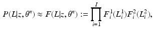
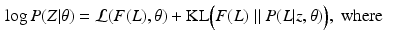
Estimation Using Graphical Modeling and Variational Bayesian Expectation Maximization: Towards a Parameter-Free Approach

Fig. 1.

(a) Real-world fluorescence microscopy images $\,z^1$ (top) and $$z^2$$

(bottom), depict the presence of protein and cell nuclei, respectively. (b) Proposed Probabilistic Graphical Model for Colocalization Estimation. Filled circles denote observed image data $\{z^1,z^2\}$ . Label images $\{L^1,L^2\}$ are hidden random variables. We estimate all parameters $\theta$ from data. The nature and strength of colocalization is modeled by parameter $\rho$ . Parameters $\beta ^1,\beta ^2$ model spatial smoothness of the labels in $$l^1,l^2$$

. In this paper, for simplicity, we use a single $\beta = \beta ^1 = \beta ^2$ . Means and standard deviations $\mu ^{\cdot \cdot }, \sigma ^{\cdot \cdot }$ model image intensities of objects and backgrounds in $$z^1,z^2$$

. (c) MAP label images $l^{1*}, l^{2*}$ , indicating object presence /absence, computed after optimal parameters $\theta ^*$ are found by VBEM. Note: this paper focuses on estimating colocalization $\rho$ using VBEM, which is crucial to several clinical and scientific studies; the MAP label images are unused by VBEM and are shown only to provide additional insights into the proposed approach.

Let $L := \{ L^1, L^2 \}$ denote a random field modeling the pixel labels of the two objects. Specifically, let

be a binary label image with I pixels $\{ L^1_i \}_{i=1}^I$ with possible label values $\in \{ +1,-1 \}$ , where

indicates the object’s presence at pixel i in

; similarly,

indicates the object’s absence at pixel i in

. We follow similar notations and semantics for

. We assume that the spatial distributions of objects are (i) smooth within each image and (ii) codependent between images. To model these properties, each pixel has intra-image and inter-image neighbors.

We introduce a neighborhood system 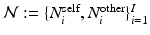$\mathcal {N} := \{ N^{\text {self}}_i, N^{\text {other}}_i \}_{i=1}^I$ , where $N^{\text {self}}_i$ and $N^{\text {other}}_i$ denote sets of neighbors of pixel i in the same image (to which pixel i belongs) and the other image, respectively. To have isotropic neighborhoods, we employ Gaussian-weighted masks w where the ij-th element $w_{ij} := \exp (- \parallel x_j - x_i \parallel ^2 / \alpha ^2)$ , where

and

are physical coordinates of pixels i and j, respectively. We use two such masks, i.e., $w^{\text {self}}$ (for intra-image smoothness) and $w^{\text {other}}$ (for inter-image colocalization) with underlying parameters $\alpha ^{\text {self}}$ and $\alpha ^{\text {other}}$ , respectively. We set $\alpha ^{\text {self}} := 2/3$ pixels to restrict the neighborhood to 2 neighbors along each dimension (we restrict the neighborhood so that $$$w_{ij} > 10^{-3}$$” src=”/wp-content/uploads/2016/09/A339424_1_En_1_Chapter_IEq35.gif”> for neighbors i, j); we found that this level of smoothness suffices for the data used in this paper. We set <IMG alt=$ to be large enough to be able to model the longest-range direct spatial interactions between the biological entities; this is application dependent and informed by prior knowledge, but the results are fairly robust to the choice of this parameter. In this paper, $\alpha ^{\text {other}} := 2$ pixels.

We model the prior probability mass function (PMF) of the label image pair L as

$\begin{aligned} P (l) := \frac{1}{Z (\rho ,\beta )} \exp \left( \sum _{i=1}^I \sum _{j \in N^{\text {self}}_i} \beta \left( l^1_i l^1_j + l^2_i l^2_j \right) w^{\text {self}}_{ij} + \sum _{i=1}^I \sum _{j \in N^{\text {other}}_i} \rho l^1_i l^2_j w^{\text {other}}_{ij} \right) \!\!, \end{aligned}$

(1)

where the normalization constant (partition function) $Z (\rho ,\beta )$ is a function of the smoothness parameter $\beta \in \mathbb {R}^+$ and the colocalization parameter $\rho \in \mathbb {R}$ . The motivation for this model is as follows. The terms involving $\beta$ are derived from a standard Ising model of smoothness on the label images. The term involving $\rho$ is novel and carefully designed as follows. First, $\rho = 0$ decouples the two label images such that P (l) can be written as

; this indicates absence of colocalization. Second, because the labels are designed to be $\pm 1$ , a positive $\rho \gg 0$ forces the interacting labels in the two images

(i.e., labels in neighborhoods of each other) towards being equal (i.e., both

or both

) to produce a high label image probability. This implies that the neighboring labels in the two images both likely indicate the presence of the objects or both indicate the absence of the objects. Third, similarly, a negative $\rho \ll 0$ forces the interacting labels in the two images to be negative of each other, i.e., the presence of the object on one image indicates the absence of the other object in the other image.

Let $Z := \{ Z^1, Z^2 \}$ denote a random field modeling the intensities of the two objects and the backgrounds. We assume that the intensities of each object are Gaussian distributed as a result of natural intensity variation, partial-volume effects, minor shading artifacts, etc. We assume that the data is corrupted by i.i.d. additive Gaussian noise. Let the intensities of the object and the background in the observed image

, where $k \in \{ 1, 2 \}$ , be Gaussian distributed with parameters $\{ \mu ^{k1}, \sigma ^{k1} \}$ and $\{ \mu ^{k2}, \sigma ^{k2} \}$ , respectively. Then, the likelihood of observing data z, given labels l, is

$\begin{aligned} P (z | l) := \prod _{i=1}^I G (z^1_i | \mu ^{1 t^1_i}, \sigma ^{1 t^1_i}) \prod _{i=1}^I G (z^2_i | \mu ^{2 t^2_i}, \sigma ^{2 t^2_i}), \end{aligned}$

(2)

where

maps the label value

to the object number, i.e.,

and

; similarly for

Let the set of parameters be $\theta := \theta _P \cup \theta _L$ , where the prior parameters are $\theta _P := \{ \rho ,\beta \}$ and the likelihood parameters are $\theta _L := \{ \mu ^{11}, \sigma ^{11}, \mu ^{12}, \sigma ^{12}, \mu ^{21},$ $\sigma ^{21}, \mu ^{22}, \sigma ^{22} \}$ . We propose to formulate colocalization estimation as the following maximum-a-posteriori Bayesian estimation problem over all parameters $\theta$ :

$\begin{aligned} \arg \max _{\rho } \left( \max _{\theta - \{\rho \} } P (z | \theta ) \right) \text {, where } P (z | \theta ) = \sum _l P (z,l | \theta ) = \sum _l P (z | l, \theta _L) P (l | \theta _P). \end{aligned}$

(3)

A novelty in our approach is that we estimate $\rho$ (as well as $\beta$ ) automatically from the data. We observe that the optimization of the parameters $\rho$ and $\beta$ is non-trivial because of their involvement in the partition function $Z(\rho ,\beta )$ that is intractable to evaluate. Furthermore, we optimize all parameters underlying the model directly from the data.

3.2 Expectation Maximization for Parameter Estimation

We treat the labels L as hidden variables and solve the parameter-estimation problem using EM. EM is an iterative optimization algorithm, each iteration comprising an E step and an M step. Consider that after iteration n, the parameter estimate is $\theta ^n$ . Then, in iteration

, the updated parameter estimate $\theta ^{n+1}$ is obtained as follows.

The E step involves constructing the $Q(\cdot )$ function

$\begin{aligned} Q (\theta ; \theta ^n) := E_{P (L | z, \theta ^n)} [ \log P (z,L | \theta ) ] \end{aligned}$

(4)

that is intractable to evaluate analytically. Furthermore, a Monte-Carlo simulation-based approximation of the expectation leads to challenges in reliable and efficient sampling; e.g., while Gibbs sampling of the label fields is computationally expensive, determining an appropriate burn-in period and detecting convergence of the Gibbs sampler pose serious theoretical challenges. Thus, we opt for variational inference and choose to approximate the posterior PMF $P (L | z, \theta ^n)$ by a factorizable analytical model

$\begin{aligned} P (L | z, \theta ^n) \approx F (L | z, \theta ^n) := \prod _{i=1}^I F^1_i (L^1_i) F^2_i (L^2_i), \end{aligned}$

(5)

where we optimize the per-pixel factors, i.e., PMFs,

to best fit the posterior. This factorized approximation for the posterior makes the $Q (\theta ; \theta ^n)$ function more tractable. We describe this strategy in the next section.

The M step subsequently maximizes the $Q (\theta ; \theta ^n)$ function over parameters $\theta$ . The E and M steps are repeated until convergence; we observe that a few iterations are suffice.

3.3 E Step: Variational Inference of the Factorized Posterior

Within each EM iteration, we use variational inference to optimize the factors underlying $F (L | z, \theta ^n)$ . To simplify notation, we omit $\theta$ where it is obvious. We rewrite

$\begin{aligned} \log P (Z | \theta )&= \mathcal {L} (F(L), \theta ) + \text {KL} \Big ( F(L) \parallel P (L|z,\theta ) \Big ), \text{ where }\end{aligned}$

(6)

$\begin{aligned} \mathcal {L} (F(L), \theta )&:= \sum _l F(l) \log \Big ( P(z,l|\theta ) / F(l) \Big ) \end{aligned}$

(7)

and $\text {KL}(A \parallel B) \ge 0$ denotes the Kullback-Leibler (KL) divergence between distributions A and B. Our goal is to find the maximal lower bound $\mathcal {L} (F(L))$ of the data log-probability $\log P (Z)$ , under the factorization constraint on F(L). We do this by maximizing $\mathcal {L} (F(L))$ , because $\text {KL}(\cdot ) \ge 0$ guarantees $\mathcal {L} (F(L))$ to be a lower bound. We perform this functional optimization by iterative optimization of each of the factor functions; this is possible because the factors are designed to be independent of each other. We now incorporate the factorized form of F(L) and, without loss of generality, separate terms involving

from the other terms. This yields

$\begin{aligned} \mathcal {L} (F(L)) = \sum _{l^1_j} F^1_j (l^1_j) \log \widetilde{P} (z,l^1_j) - \sum _{l^1_j} F^1_j (l^1_j) \log F^1_j (l^1_j) + \text{ constant },\end{aligned}$