(1)
Intelligent Systems Research Centre, University of Ulster, Londonderry, UK
2.1.1 Block Design
2.1.2 Random ER Design
2.1.3 Phase-Encoded Design
2.5.5 AR(1) Model
2.5.6 AR(q) Model
2.6.4 Permutation/Random Test
Abstract
As many other scientific experiments, functional magnetic resonance imaging (fMRI) study has multilevel hierarchical nature. For example, for a single voxel in the brain, fMRI response is from i voxel position, in j run, of k subject. Therefore, a mixed effect model should be employed for the analysis. In framework of general linear mixed model (GLMM), both first and higher levels of the model parameters can be estimated using iterative schemes for the fMRI study. However, this is not practical for fMRI data analysis because of the computational burden of fitting GLMM at every voxel that is very expensive. As a result, most methods adopt a two-stage model method, and at the first stage, variance and effect from the first-level analysis are estimated for the second-/higher-level fMRI data analysis. In this chapter, we will focus on these variance and regression parameter estimation. Firstly, we present the method for fMRI experimental design, and then we introduce statistical methods for fMRI activation detection. A general linear model (GLM) for the activation detection is introduced. Because the residual terms of the linear model is autocorrelated, an autoregression (AR) model is adopted for correcting the model estimation error. After the fMRI signal is fitted with the GLM-AR model, we detail statistical inference method for activation detection. Finally, we present false discovery rate (FDR) and family-wise error (FWE) algorithms for the threshold correction.
Keywords
BOLD-fMRIfMRI experimental designGeneral linear model (GLM)Autoregression (AR)Threshold correctionActivation detectionMatrix inversion2.1 fMRI Experimental Design
The first step for processing any functional data is to understand the experimental design, and fMRI data analysis is no exception. In fact, a good fMRI experimental design is essential for the study since it not only provides the interpretable results of the scientific questions we want to address but also offers easier way to analyze the data. Because blood-oxygen-level-dependent (BOLD) response relies on the sluggish cerebral blood flow, this makes the functional magnetic resonance imaging (fMRI) experimental design different and, certainly, much harder than other types of experimental design. Therefore, many theories such as statistics, mathematics, and system theories have been applied to design fMRI experiments and analyze fMRI data. For example, if we regard the human brain as a system [1, 2], then the purpose of experimental design is to devise a system input. Since we know the predefined system input and system output, i.e., BOLD-fMRI response, we can infer what is inside the brain in response to this particular stimulus (system input). The purpose of fMRI activation detection is, therefore, to find the significant relationship between system input (experimental design or external stimuli) and fMRI response (system output). Although there are many types of fMRI experimental design available, three types of designs are commonly in use for fMRI studies currently, i.e., block design, (random) event-related (ER) design, and phase-encoded design. We will introduce these designs briefly in this section.
2.1.1 Block Design
Perhaps, block design is the simplest and most frequently used experimental design for fMRI study. In a typical block design, there is a control condition block with one or more task blocks, and the control block and task block appear alternatively. The duration of each block is about 10–20 s. The length of these blocks can be equal or unequal. If the length of each condition block is equal, then it has additional advantage, i.e., Fourier analysis method can be applied straightforward because the stimuli change periodically.
Figure 2.1 shows one example of block design for emotional face processing. In this design, there is one white cross fixing control condition and three face/task conditions, and each block appears alternatively. The task conditions include neutral faces, sad faces, and happy faces. There are five faces with the same type of presentation within each block, and the duration of each face is 2 s.
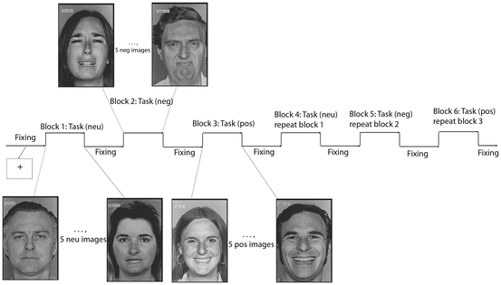

Fig. 2.1
An example of block design: emotional face processing experiment. One example of standard block design paradigm where on and off length of each block is equal: pos, neg, and neu denote positive, negative, and neutral face, respectively. Fixing is eye fixation to the center of the screen
In this experimental design, we can study the brain response to the face stimuli by comparing all the face condition response with the white cross fixing condition. In addition, we are able to address the emotional effect by comparing happy/sad face response with the neutral face condition. Finally, the question of the brain region difference in response to happy and sad faces can also be answered using statistical methods.
Ideally, it is always better to collect as many brain fMRI responses as possible. However, because subjects cannot maintain their positions in the scanner for a long time, we often take each functional run last 6–20 min. If more fMRI time slots are available, we can employ repeated run measure methods to collect more data from the same subject.
It should be mentioned that during the fMRI experiments, subjects are asked to perform certain task which may be irrelevant to stimuli but to help subject to keep awake in the scanner.
2.1.2 Random ER Design
Another type of fMRI experimental design commonly in use is ER design. It has been used for many studies including, but not limited to multisensory, visual/auditory psychophysics, perception learn, and neuronal adaptation studies. As the name indicated, in the random design, each event or condition/block will appear randomly so that the subject cannot guess what the next stimulus is during the experiment. It is worthwhile to mention that the rapid ER design with randomly select interstimulus interval belongs to ER design, and it has been becoming popular for fMRI studies. When using this type of experiment design paradigm, because hemodynamic delay of the cerebral blood flow, it should be kept in mind to leave enough time interval between two events [3].
One example of random ER design paradigm which was used for emotional face processing study is shown in Fig. 2.2. In this ER design, we include four conditions, e.g., three task conditions (neutral, sad, happy face stimuli) and one control stimulus (white cross fixation) condition. The presentation of each task condition is randomly selected, and there is a white cross eye fixation control condition after each neutral, sad, and happy faces stimuli condition. The duration of white cross is varied according to the duration of the face stimulus. For instance, if a single face which takes 2TR (TR is the scanner repetition time, in this example experiment, we set TR = 2 s) to present, a white cross stimulus with 4TR duration is displayed subsequently. We represent this task as event block 1 in Table 2.1, and it takes 6TR to finish the task in total.


Fig. 2.2
An example for random ER design paradigm. X-axis is time (unit TR). In the y-axis, 1, 2, 3, 4 denote white cross fixation, neutral, sad, and happy face stimulus presentation, respectively
Table 2.1
Task assignment for random ER emotional facial processing study
Face type | Neutral | Sad | Happy | No. of TR(2 s) |
|---|---|---|---|---|
Event block 1 | 1,2,3 | 4,5,6 | 7,8,9 | 9 × 6 = 54 |
Event block 2 | 10,11,12 | 13,14,15 | 16,17,18 | 9 × 10 = 90 |
Event block 3 | 19,20,21 | 22,23,24 | 25,26,27 | 9 × 13 = 117TR |
Total time | 261TR = 8 min 42 s |
The second event block in Table 2.1 is a double face stimuli (same type of the stimulus presented two times, i.e., both happy/sad/neutral faces, but different person face) presentation, which needs 4TR (2TR + 2TR) for faces presentation and 6TR for white cross displays.
The third type of event block is a triple stimuli presentation, which includes 6TR (2TR + 2TR + 2TR) for the same type of face presentation and 7TR for white cross display. The role of the white cross is to separate face condition with other types of face stimuli tasks.
For each condition and each case, we have three repetitions. It is easy to see that the design is balanced, i.e., the total number of each condition is the same. We arrange each event from 1 to 27 as shown in Table 2.1, and then we randomly select each number; as a result, each event block will appear randomly. Therefore, the interval between each even block is randomly determined accordingly. The total time for this experiment is 8 min 42 s, as given in Table 2.1.
We may want to study the correlation between brain activation and behavioral task; we need to record the task performance during the MRI scan for the analysis. In addition, we may want to do additional behavioral tests after MRI scan, for example, in this experiment, during the fMRI experiment in the scanner, and we ask the subject to remember the face and corresponding name for a memory test after MRI scan.
To help understand the experimental design, we give one typical fMRI response (Fig. 2.3) from the experimental design paradigm as shown in Fig. 2.2. In Fig. 2.3, the blue thin solid curve denotes the normalized experimental design in Fig. 2.2, the dotted curve represents the fMRI response, and the red thin curve displays the model fitting for the response when comparing faces with white cross fixation condition (data is from Appendix D). It is obvious that the fMRI response follows the experimental design, suggesting that there is activation at this particular brain voxel position.


Fig. 2.3
An example of fMRI response for random event-related (ER) block design for emotion study. T is T statistical test
2.1.3 Phase-Encoded Design
Another regularly used fMRI experimental deign is phase-encoded design. In contrast to block and ER designs, although phase-encoded design is less frequently in using, it has been applied successfully in visual retinotopic mapping studies [4–6] and proved to be another effective way to study visual cortex.
The idea of this type of design is to present a travelling wave (shift block) type stimulus in which stimulus changes continuously, without obvious interruption. For example, in visual retinotopic expanding ring stimulus, we change the position of the checkerboard pattern slowly over time, a flicker checkerboard color ring stimulus growing from small size (a) to big (d) as shown in Fig. 2.4. Then another small ring appears in the central of the stimulus to replace the largest ring stimulus in Fig. 2.4d, and the whole process repeated itself. This is the eccentricity stimulus for retinotopic mapping study. We also can create a contracting ring, in which the size of the ring changes from biggest (d) to smallest (a). Combining with phase-encoded wedge (polar angle) stimuli (Fig. 2.5), we can calculate the visual sign map and define the boundaries of the early visual cortex accordingly [4–6].


Fig. 2.4
Phase-encoded expanding ring stimulus for visual cortex retinotopic mapping study. (a–d) Ring expanding from small (a) to big (d)

Fig. 2.5
Phase-encoded polar angle (wedge) stimulus for visual cortex retinotopic mapping study. (a-b) Different angle of rotated wedge stimuli
Figure 2.5 shows the polar angle stimulus for the retinotopic mapping study. Typically, it consists of a rotated wedge, whether clockwise or anti-clockwise rotation. When doing the experimental in the scanner, the subjects are asked to keep eye fixation at the center of the stimulus and perform certain task, i.e., detecting the regular black/white (Fig. 2.5a), blue/yellow (Fig. 2.4c), and red/green (Fig. 2.5b) patterns in the stimulus.
Based on the idea of phase-encoded design, we extended the ring stimuli to spatial frequency [7] and contrast sensitivity perception [8] stimuli for visual cortex studies. For instance, in the phase-encoded spatial frequency design, the spatial frequency changed periodically either from medium to low or from low to medium (Fig. 2.6) in which the spatial frequency of a sinusoidal checkerboard stimulus was gradually varied from 0.5 to 6 c/d over a 1 min period. The temporal frequency of the checkerboard stimulus was 8 Hz. This involved a smooth and gradual change in the spatial frequency of the sinusoidal checkerboard evenly throughout the field. A central fixation point was provided. The stimulus and design matrix are depicted in Fig. 2.6c. The attention of the subjects was controlled using a target detection task as described above for the block design. The advantage of this design is that the stimulus changes smoothly, rather than dramatically changes as in block design, and the fMRI response will change smoothly accordingly which is easier to deal with using Fourier analysis method. Because from Fourier analysis, we know that the periodical triangle stimuli (Fig. 2.6c) can be approximated by a set of sinusoidal functions. The fundamental frequency sinusoidal function of the triangle stimulus can be employed to model the fMRI response (Fig. 2.7). In Fig. 2.7, the dotted curve indicates the fMRI response (data is from Appendix E), and the solid curve denotes the fundamental frequency of the triangle wave (Fig. 2.6c) as a model for hemodynamic response function (HRF).


Fig. 2.6
Phase-encoded design for spatial frequency perception. (a) An example of high spatial frequency stimulus. (b) An example of low spatial frequency stimulus. (c) The stimuli presentation paradigm. cpd denotes cycle per degree

Fig. 2.7
An example of fMRI response to the phase-encoded spatial frequency experimental design
2.2 fMRI Data Preprocessing
After fMRI data have been collected, we need to preprocess the data to correct subject head motion, register individual subject brain image to a standard template for comparison, and normalize the fMRI time series to remove the position shift in the response.
2.2.1 fMRI Data Motion Correction
In a typical fMRI experiment, we collect not only functional data but also structural MRI data for brain activation localization, visualization, and comparison with other subjects. We may also want to compare different subject from different image modalities; as a result, we need to register different subjects to a standard template for comparison. To achieve these goals, we need to register functional data to a high spatial resolution structural image, which needs to be matched to the standard template for group comparison. Image registration methods [9, 10] for these purposes have been developed, and there is a lot of software packages freely available.
For functional images, we perform image registration to correct head movement during data collection within each run and across different runs. In the literature of image registration, many methods have been developed. For example, correlation method, linear and nonlinear least squares methods, and mutual information methods have been developed. In our study for fMRI data preprocessing, dynamic motion correction for functional image time series for each run and for different runs was realigned at the same time by using the fmr_preprocess within MINCtools (http://www.bic.mni.mcgill.ca/ServicesSoftware/HomePage) with default parameters for three-dimensional Gaussian low-pass filtering [11].
2.2.2 fMRI Time Series Normalization
After motion correction, the next step is to normalize the fMRI time series to exclude the baseline shift in the analysis. There are two ways to normalize fMRI time series, i.e., temporal and spatial normalization methods. For the spatial normalization, we need to segment the brain region from the image background and using the voxels within the brain region for normalization. For the temporal normalization, we normalize the fMRI response longitudinally, i.e., if we employ x i to denote the fMRI signal at time point (fMRI image frame) i, then we use

to normalize the signal, where  is the mean value of the time series and
  is the standard deviation of the time series.

(2.1)
 is the mean value of the time series and
  is the standard deviation of the time series.
Figure 2.8a shows one example of fMRI image intensity time series from previous study [12] which adopted a typical standard block design (see Appendix F for data collection). Figure 2.8b shows the corresponding temporal normalization results using Eq. (2.1). The thin solid curve is the fundamental frequency model for HRF, and the thick solid curve denotes the fitted results. Comparing Fig. 2.8a with dotted curve in Figure 2.8b, it is easy to see that although the magnitude of these two curves is different (the baseline in Fig. 2.8b has been removed), the shape is similar, suggesting fMRI normalizing step maintains the temporal information of the signal changes. In Figs. 2.3 and 2.7, the solid curves represent the temporal normalized fMRI responses.
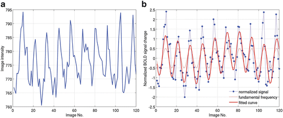

Fig. 2.8
Temporal normalization of fMRI response for a standard block design. (a) Raw fMRI image intensity time series. (b) Normalized fMRI signal
2.3 Activation Detection: Model-Free and Model-Based Methods
After fMRI time series have been corrected for head motion and normalized, it is ready for activation inference using statistical methods. Methods for fMRI activation detection can be classified into two broad categories: one is the model-free method and the other is model-based method. For the model-free method, we do not need to build any fMRI response models, i.e., HRF beforehand for activation detection. While for the model-based method, we need to build a model for the analysis. In this chapter, we will introduce both model-free and model-based methods for activation detection at first-level analysis.
2.3.1 Model-Free Method: Two Sample t-test for Activation Detection
The simplest model-free method for activation detection is to compare the task fMRI response with the control condition response. The idea of this method is to compare the mean value of the neuron population response from task condition and control condition. This can be done based on the assumption that the task stimulus response and control condition response are two independent variables, randomly sampled from an approximately normal distribution. Therefore, we can apply a two-sample t-test as [13]

for activation detection, where variance s can be calculated as

where  and
and  are the mean values of task stimulus response and control condition response. The degree of freedom (df) for the hypothesis test is k = n 1 + n 2 − 2. n 1 and n 2 are the total number of time point from the task condition and control condition, respectively. The next step is to compare the calculated T value with k df with the critical t value from the t distribution table at the chosen confidence level and decide whether to accept or reject the null hypothesis. Reject the null hypothesis when the calculated T value is larger than the critical T value, e.g., declare activation at this voxel.

(2.2)

(2.3)
 and
and  are the mean values of task stimulus response and control condition response. The degree of freedom (df) for the hypothesis test is k = n 1 + n 2 − 2. n 1 and n 2 are the total number of time point from the task condition and control condition, respectively. The next step is to compare the calculated T value with k df with the critical t value from the t distribution table at the chosen confidence level and decide whether to accept or reject the null hypothesis. Reject the null hypothesis when the calculated T value is larger than the critical T value, e.g., declare activation at this voxel.
The major advantage of this method is simple, as the t-test method does not require any prior defined HRF model for activation detection. It only needs the information of the stimuli duration and starting time. However, this method is based on the assumption that the individual fMRI signal is i.i.d., and this is not realistic because of the nature of the hemodynamic response of the blood flow. Moreover, this method does not take fMRI response slow drift into account, which can lead to estimation error.
2.3.2 Correlation Analysis Method
Correlation analysis is another model-free method for activation detection [14]. To apply correlation analysis method for activation detection, one needs to select a seed point time series which is supposed to be activated for this particular brain region in response to the stimulus. Then we correlate this fMRI time series from the predefined seed region with the rest of the brain. We obtain the correlation coefficient (CC) and use CC to determine whether it is significantly correlated or not. We can also covert CC to Z score and t value for significant inference. Pearson correlation coefficient is often adopted for the calculation as

where x 1i is the seed region time series and  is the mean value of the fMRI series. It can also take the form of averaged time series from a region; x 2i is the fMRI time series from the rest of the brain,
  is the mean value of this series, and n is total number of time series.

(2.4)
 is the mean value of the fMRI series. It can also take the form of averaged time series from a region; x 2i is the fMRI time series from the rest of the brain,
  is the mean value of this series, and n is total number of time series.
The advantage of this method is that it is simple to implement; however, this method is also easy to be disturbed by the slow drift, especially, in the seed region. Moreover, if the seed region is not selected properly, this can lead to large estimation error for activation detection. Although linear and quantic shifts have been incorporated to eliminate the slow drift effect, brain activation detection using this method is highly dependent on the predefined seed region. Human cerebral anatomy knowledge is also needed to decide the seed region/voxel.
2.4 Models for Hemodynamic Response Function and Drift
Because of the limitations of model-free methods for fMRI activation detection, model-based method such as general linear model (GLM) has been developed and used for activation detection. The first step to apply model-based method is to build an HRF model for the fMRI response. Currently, there are mainly three HRF models for fMRI activation detections, i.e., fundamental frequency of Fourier component model, two-gamma function model, and boxcar function convolve with Gaussian function model.
2.4.1 HRF Models for Activation Detection
If the stimuli in the experimental design are changing periodically and the duration of each block condition is equal (Figs. 2.7, 2.8b, and 2.9), then fast Fourier transformation (FFT) method can be applied to model the HRF from fMRI response [15]. This is because the periodical square block wave can be approximated by the fundamental frequency of the sinusoidal wave (e.g., Fig. 2.8), and it is a powerful way to study experimental design with periodical change stimuli. The sine wave function has the form


where θ is the delay/onset or phase of the response that is estimated using the FFT method; ω is the angular frequency; ω = 2πf, where f is the frequency of the stimulus; and a is the magnitude. The algorithm to estimate parameters θ and a in Eq. (2.5) is as follows:

Fig. 2.9
One typical fMRI response and its fundamental frequency model for HRF from phase-encoded retinotopic mapping study. The block function (thin solid curve) and the fundamental frequency of the response (thick solid curve); the estimated onset for the first block is 8 from the FFT analysis

(2.5)
1.
2.
Get the angle and magnitude of the signal from FFT.
3.
Obtain the angle and magnitude information corresponding to the fundamental frequency; this angle information is used to estimate the fMRI response delay.
4.
Compute ifft (inverse FFT) using fundamental frequency magnitude information.
5.
Adopt only the real value of the inverse FFT transformation to get the HRF fundamental frequency model, i.e., f t,1 in Eq. (2.5).
Based on this algorithm, we obtain the estimated HRF model displayed as solid red curve in Fig. 2.7 (six cycles), Fig. 2.8b (ten cycles), and Fig. 2.9 (six cycles).
Another widely used function to model the BOLD-fMRI HRF is two-gamma function (Fig. 2.10a, b). To estimate the two-gamma function adaptively, we need to estimate the delay/onset of the function by the FFT analysis (Eq. (2.5)) or cross correlation analysis. Then, a two-gamma function is built according to the following equation [16]:


Fig. 2.10
Two-gamma function model for HRF. (a) The two-gamma function model for the response with varying parameter a 1; (b) The two-gamma function for the response with varying parameters a 2 and b 2

(2.6)
Stay updated, free articles. Join our Telegram channel

Full access? Get Clinical Tree


