(4.1)
The b-factor in this equation captures all the relevant scanning parameters and was introduced to take abstraction of them [2]. In general, it can be seen as the amount of diffusion weighting that is applied; i.e. how sensitive the acquisition is to diffusion. Its value is typically set and reported in s/mm2. As a realistic value for our simple experiment at hand, we could have chosen e.g. 800 s/mm2. We can rewrite this equation so it becomes
(4.2)
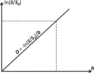
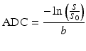
Fig. 4.1
In case of free diffusion (e.g., in a glass of water, or CSF in the ventricles of the brain), the plot of − ln(S/S 0) in function of b-value is a straight line through the origin. One point (grey short dashed lines) is enough to fully fix this line. It requires two images (S and S 0) as well as knowledge of the b-value used to acquire S. The slope of the resulting line equals the self-diffusion coefficient D

(4.3)
Conclusions
We are now able to calculate the self–diffusion coefficient D of free water (be it in a glass or as CSF in the ventricles), using measurements from a MR scanner and the Stejskal-Tanner equation. The minimum requirements are a nondiffusion-weighted image (S 0), a diffusion-weighted image (S) and knowledge of the b-value that was used for performing the acquisition of the diffusion-weighted image.
The Apparent Diffusion Coefficient
Apparent Complications
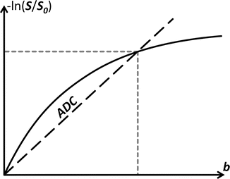
Feeling confident about the newly gained ability to obtain D from the two images we acquired of our brain, we also attempt to perform the same calculation in a voxel of gray matter. Suddenly, however, we are confronted with a resulting value of about 0.9 × 10⁻³ mm2/s. Apparently, the self-diffusion coefficient of water has changed, just because we measured it in the gray matter. Maybe something went wrong with the scan? We perform the acquisition again for a couple of different b-values. Carefully dotting out the obtained values of − ln(S/S 0) in function of b and connecting everything loosely by hand, we obtain a curve such as the one depicted in (Fig. 4.2). Apparently, the self-diffusion coefficient of water now even changes in function of our chosen acquisition parameters. Using Eq. (4.3) to calculate D equates to connecting a certain measured point on this curve with the origin by a straight line (as shown in Fig. 4.2 ) and assuming its slope still equals D. Since the obtained values are clearly lower than expected and they also seem to vary in function of b, such a value is referred to as an apparent diffusion coefficient (ADC) [3]. It’s calculated from the measurements in exactly the same way as D:
To understand the behavior of the obtained ADC in regions containing tissue (e.g., gray matter), we need to look into how the acquisition of a diffusion-weighted image works. An existing (e.g., T2-weighted) sequence is modified by adding a couple of diffusion-sensitizing gradients. By taking abstraction of any complicated MR physics, we could say the MR scanner actually performs a simple experiment in each voxel: it takes a snapshot of all the water molecules, waits a bit, and then takes another snapshot. During the short waiting time, however, the molecules have the opportunity to diffuse a bit. Per consequence, a relative displacement of each molecule can take place in between both snapshots. The expected signal of the original (e.g., T2-weighted) sequence is attenuated in function of the amount of displacement of all water molecules in the voxel (as well as the amount of applied diffusion weighting). From the measurements of such an experiment (relative to a nondiffusion-weighted image), the Stejskal-Tanner equation is able to reliably calculate D… if and only if nothing disturbs the experiment. However, in tissue, such as gray matter, there are cell membranes all over the place. Because the water molecules happen to bump into the cells—i.e., they are hindered—they have a harder time to diffuse further away during the experiment. Water inside the cells may even be restricted to a confined space. And thus, our calculation of D will apparently yield a lower outcome, which is why we call it the ADC instead. The time the experiment allows the molecules to diffuse is one of the parameters that makes up the b-value. It’s easy to imagine that a larger diffusion time will allow more molecules to hit some of these cell membranes. Hence, the effect of the hindered/restricted diffusion on our measurement will increase with b-value; yet another reason to refer to the outcome of our calculations using the term “ADC”. This is also illustrated in (Fig. 4.3 ): using a larger b-value renders the measurement of S less sensitive to (truly) free diffusion, in favor of hindered/restricted diffusion. As such, S will be less attenuated and the value of − ln(S/S 0) will be smaller than expected, yielding a downward curvature when plotting − ln(S/S 0) in function of b. This finally leads to an important property of the ADC in tissue, as indicated in (Fig. 4.3): using a higher b-value results in a lower ADC.
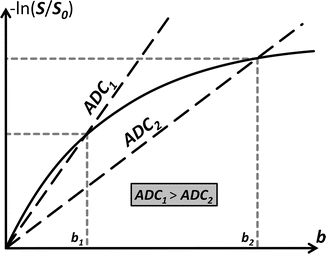
Fig. 4.2
In case of hindered/restricted diffusion (in tissue, e.g. the grey matter of the brain), the plot of − ln(S/S 0) in function of b-value is a curve through the origin. Based on one point (grey short dashed lines), we can calculate an apparent diffusion coefficient (ADC). Just like D, it equals the slope of the line that connects this point to the origin (black long dashed line)
(4.4)
Fig. 4.3
The ADC is dependent on the b-value used to acquire S. Due to the downwards curvature of the plot of − ln(S/S 0) in function of b-value, a larger b-value results in a lower ADC. An explanation lies, e.g., in the fact that increasing the diffusion time allows more molecules to bump into cell membranes. This will on average decrease their final displacement, resulting in a reduced amount of attenuation of S and finally leading to a lower value for − ln(S/S 0) than expected in a free (non-hindered/restricted) environment
Apparent Advantages
At this point, you might start to wonder what the point is of trying to find out D in voxels containing tissue, only to end up having to deal with a deceiving ADC instead. However, you have to look at it from the bright side: we now effectively have access to a probe that tells us something about these cells that hinder/restrict diffusion. That’s right: even though our voxel size might be quite crude (2 × 2 × 2 mm3 or larger is not unusual), the measured values are sensitive to differences in structure at a micrometer scale! We are not interested in the ADC for the purpose of quantifying diffusion itself, but rather to investigate properties of the tissue that apparently caused the diffusion process to behave in the way that we measure.
Before moving on, let’s investigate one more property of the ADC that teaches us something else about its capacity in distinguishing different tissues. Consider the setting in (Fig. 4.4): it presents again − ln(S/S 0) in function of b, but this time for measurements at two different locations (e.g., in the brain). Looking at the plots and applying what we just learned, we can safely say that the voxel at position p g contains more hindering/restricting tissue than the voxel at position p f. The former voxel’s plot shows greater curvature, while the latter better approximates the straight line we would expect in case of free diffusion. Due to this difference in curvature of both plots, the relative difference in magnitude of − ln(S/S 0), and thus also ADC, increases for larger b-values. In other words, using a larger b-value results in a better contrast when calculating an ADC map. This fact of course begs the question why we should still limit ourselves to a certain b-value. That is, why not use an absurdly high b-value for maximal contrast? The two most important factors that generally contribute to the b-value are the strength of the applied diffusion-sensitizing gradients and the time that we allow the water to diffuse during the experiment. The former is limited by what we can achieve with available hardware. The latter is fully under our control. Allowing a too long diffusion time, however, might result in other more macroscopic motion to be captured and thus confounding our measurements. Even if this would not be the case, we also have to recall that S only decays further in function of b-value (remember Eq. 4.1 again?). The noise level of our measurements, on the other hand, does not decrease; that is, using a higher b-value yields a lower signal–to–noise ratio (SNR)!
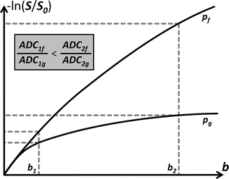
Fig. 4.4
The contrast of the ADC, e.g., between two different tissues at voxel positions p f and p g, is dependent on the b-value used to acquire S. Due to different tissue properties, both plots of − ln(S/S 0) in function of b-value show a different curvature. The tissue at p f imposes less hindrance/restriction on the diffusion as compared to the tissue at p g and thus the accompanying curve is closer to a straight line. Hence, ADCf is larger than ADCg for a given b-value. Increasing the b-value also results in an increase of the relative difference between both ADC values, i.e., an increase of contrast
Conclusions
We have learned why the MR measurements in combination with the Stejskal-Tanner equation are not suited to calculate the true self-diffusion coefficient of water in voxels containing tissue, e.g., where diffusion is hindered or even restricted. The obtained apparent diffusion coefficient (ADC), on the other hand, can provide interesting information about the microstructure of the tissue under investigation. The minimum requirements for obtaining it are again a nondiffusion-weighted image (S 0), a diffusion-weighted image (S) and knowledge of the b-value that was used for performing the acquisition of the diffusion-weighted image. The ADC is, however, dependent on the b-value: a higher b-value results in a lower ADC. It also improves the contrast (e.g., of the ADC map), but at the cost of a reduced SNR. Due to these dependencies, interpreting/reporting the ADC only makes sense when the b-value is also specified. Finally, comparing ADC values or maps originating from acquisitions with different b-values does not make a lot of sense.
Gradient Directions and Anisotropy
Anisotropic Complications
Up to now, we’ve been silently ignoring yet another important fact that will complicate everything even more. It concerns that diffusion-sensitizing gradient: it’s about time we started taking into account that it’s applied along a certain direction. Nothing to worry about, if it were not for the fact that our measurements are only sensitive to diffusion along this direction. Actually, that is not fully correct; it’s better to say that they are only sensitive to diffusion with a component along this direction. Before we start talking further about directions, let’s settle on some reference frame. We define three (perpendicular) axes through the brain as follows: x runs from left to right, y from back to front, and z from bottom to top. So suppose we would apply the diffusion gradient along the direction of x, what are the implications then? It basically means that the measurements are fully sensitive to diffusion along x, but gradually less sensitive to diffusion along directions that increasingly deviate from x, up to the point where they are completely insensitive to diffusion along directions perpendicular to x (i.e., directions in the yz-plane).
But why should we worry about directionality of diffusion anyway? In our earliest experiments with a glass of water or CSF in the ventricles, we shouldn’t: diffusion takes place equally in all directions. In tissue randomly containing cells—imagine a bunch of spherical cells packed together—diffusion is hindered and restricted, yet probably more or less equally in all directions. So again, there’s nothing to worry about: as we are in both cases studying isotropic measurements, it is sufficient to only measure along a single direction. Our findings (e.g. calculating the ADC) should have been the same for measurements along any other direction. But let’s consider the more interesting case of the white matter in the brain: it consists of long coherent bundles of axons, almost resembling a bunch of cylindrical tubes packed closely together (see Chap. 3). One can imagine that water molecules in between and inside these tubes have an easier time diffusing along them rather than perpendicular to them. We thus say that diffusion in the white matter is anisotropic.
But how relevant is this? Is this anisotropy large enough to be measured; i.e. can we see it in our diffusion-weighted images? To answer this question, we’ll introduce some real data. In (Fig. 4.5), we start by presenting a classic T1-weighted and T2-weighted image for reference. Next is the nondiffusion-weighted image: it’s again a T2-weighted image, but it already shows the lower spatial resolution at which DWI datasets are typically acquired. In this case, the voxel size equals 2.2 × 2 × 2 mm3. Because the image is not diffusion-weighted, but it is acquired as part of a DWI dataset, we also sometimes (informally) refer to it as the “B0” (it equals a diffusion-weighted image with a b-value of 0). For convenience, we already applied a whole brain mask to it. On the second row of (Fig. 4.5), three diffusion-weighted images (DWIs) are shown (also masked). They were all acquired using exactly the same amount of diffusion weighting: b = 800 s/mm2. The diffusion-sensitizing gradients are, however, applied along different directions: respectively along the direction of x, y and z. Differences in contrast can clearly be seen, which consequently confirms that we will have to account for anisotropy in our measurements .
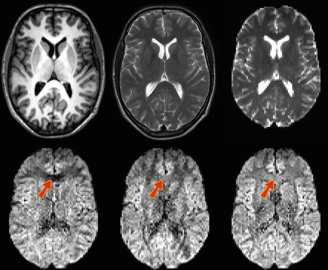
Fig. 4.5
Top row: T1-weighted image, T2-weighted image, B0 image (“diffusion-weighted image” with a b-value of 0, i.e., non diffusion-weighted). Bottom row: diffusion-weighted images (DWIs) acquired by applying gradients along the direction of x, y and z. The arrows indicate a region in the genu of the corpus callosum (GCC), where the anisotropy can be easily seen and understood
Anisotropic Advantages
Just as when we introduced the ADC, we’ll also try to use this fact to our advantage: we now have access to a probe that might even provide us with information on the anisotropy of the microstructure that hinders and restricts the process of diffusion. Applying what we have learned from this chapter up to this point, let’s see if we can already figure out something useful from these three diffusion-weighted images. Consider the indicated region in the genu of the corpus callosum (GCC ) : it has a low DWI–intensity along x, but a (relatively) higher DWI–intensity along y and z. Because we know that more diffusion causes increased decay of S (the DWI-intensity), we can conclude from these images that there is more free diffusion along x, while there is more hindrance and restriction along y and z. Translating this to “reality”, we might infer that a bundle of tubelike axons runs along the left–right axis in this region, connecting both hemispheres of the brain. Note that we are applying inductive reasoning here: we know that such a left-right oriented structure would result in such a pattern of diffusion and thus also such DWI measurements along these three directions, yet we reason that the latter measurements were effectively caused by the former structure. Considering we only measured along three directions, that’s a pretty strong conclusion. Of course, inherently we might have also applied possible anatomical knowledge and the fact that a structure along this direction makes sense considering the spatial/anatomical neighborhood of the region (i.e., the region is in between both hemispheres ).
Getting a Grip on the Information Overload
In practice, however, we will typically perform the acquisition using more than three different gradient directions. In the previous example, we were just lucky that the structure under investigation accidently happened to run along one of the three mutually perpendicular directions that we sampled. If it would instead be running at any other oblique angle, these three measurements would clearly be inadequate to determine its direction. In our experiment at hand, however, we actually acquired DWIs for a total of 45 different gradient directions! The specifics of such an acquisition are presented in the gradient table, that contains one row for each acquired image, representing its gradient direction and b-value. The gradient table for our current experiment is provided in (Fig. 4.6 ). As it was already quite tedious to infer information by mentally combining three images, considering 45 DWIs all at once is nearly impossible. To begin with, we will no longer visualize the original DWIs, as they are still only representing a (partially) decayed T2-weighted signal. Because of this, these DWIs suffer so-called T2 shine–through: a higher intensity might not (only) result due to hindered/restricted diffusion; it might also be caused by an originally high T2 intensity (e.g., in areas containing CSF). Therefore, it is more evident to consider DWIs after normalization by the B0 (i.e., the normalized measurements “S/S 0”). Such normalized versions of our original DWIs for the three x, y, and z gradient directions are shown in (Fig. 4.7 ). Next up is the actual challenge of visualizing the information of all 45 normalized DWIs in a conveniently organized way. Rather than showing 45 separate images, we could try to combine all information of each single voxel and visualize it within that particular voxel. Since the different values of S/S 0 are a function of the gradient direction, a spherical polar plot is the perfect candidate for the job. In such a plot, the radius of a sphere is locally manipulated to equal the function value at that three-dimensional angle. We also smoothly interpolated the values between the 45 directions in order to achieve the final visualization in (Fig. 4.7). Note that, due to the multitude of information on display, we have to zoom in up to a reasonable level to show everything with the required amount of detail. We choose to further focus on the region of the GCC that was the subject of our earlier thought experiment. Furthermore, a little extra color was added to the plot: each point on the surface of the spherical polar plots is colored according to its direction: red is assigned to x, green to y and blue to z. In (the middle of) the GCC, we spot larger values for green (y) and blue (z), and smaller values for red (x). By linking larger values to hindrance/restriction, we can thus confirm our hypothesis of an axonal bundle connecting left and right.
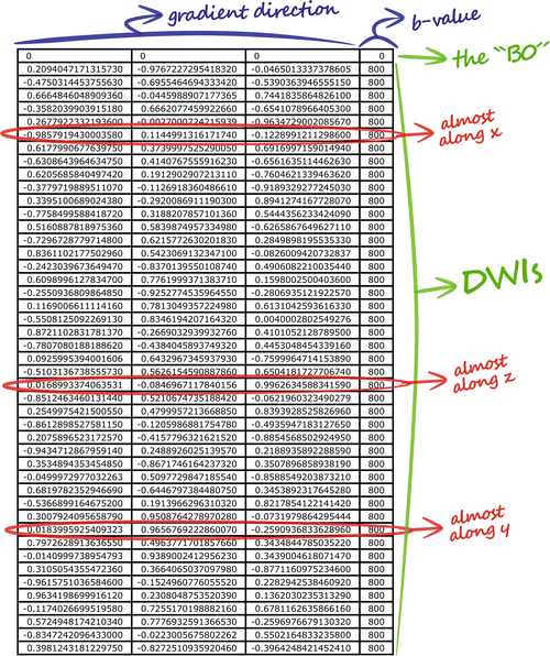
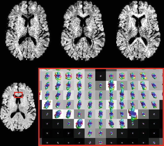
Fig. 4.6
The gradient table contains one row for each acquired image. The x, y and z components of the gradient direction are provided in the first three columns, while the b-value is given in the last one. A b-value of 0 indicates a B0 image; the gradient direction is irrelevant in such a case. The red encircled rows refer to the DWIs presented in Fig. 4.5
Fig. 4.7
Top row: DWIs for the x, y, and z gradient directions, after normalization by the B0 (i.e., the normalized measurements “S/S 0”). Bottom row: Spherical polar plots of the normalized DWI values in a region of the GCC, overlaid on a map of the average normalized DWI value
Associating larger values with less diffusion still feels a bit awkward, to say the least. So why don’t we simply employ the ADC values? Easy enough: just calculate the 45 ADC maps from the normalized DWIs using Eq. (4.4). We present these maps—again for the three x, y, and z gradient directions—in (Fig. 4.8). This time, larger values equal more free diffusion. We can just as well create a spherical polar plot of the 45 ADC values in each voxel, which is again provided for the GCC region in (Fig. 4.8 ). Larger values are now conveniently oriented along the direction of the greatest amount of free diffusion, and colored accordingly. Finally, remember that property of the contrast increasing with b-value? Of course, it also applies for measurements (and ADC values) acquired using different gradient directions: using a higher b-value will increase the contrast in these spherical polar plots. However, as we reasoned before, the SNR will also drop.
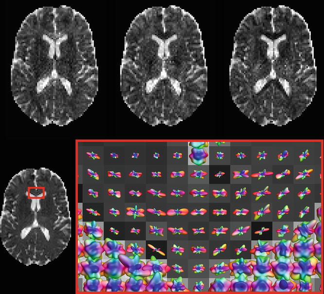
Fig. 4.8
Top row: ADC maps for the x, y, and z gradient directions. Bottom row: Spherical polar plots of the ADC values in a region of the GCC, overlaid on a map of the average ADC value
Conclusions
We started taking into account the fact that the diffusion-sensitizing gradient is applied along a certain direction. The resulting DWI measurement is only sensitive to diffusion with a component along this direction. From DWIs acquired using different gradient directions, we could conclude that anisotropic diffusion takes place in the white matter up to a measurable extent. Again using this to our advantage, we now have a probe for the anisotropy of microstructure in each voxel. There are different ways to visualize data resulting from acquisitions using many different gradient directions, yet the most convenient option was a spherical polar plot of the ADC values in each voxel: such a visualization shows larger values along the direction exhibiting the greatest amount of free diffusion. Optional color coding is typically done according to a directional scheme: red for x (left–right), green for y (back–front), and blue for z (bottom–top). The requirements for investigating the anisotropic nature of diffusion are a B0 (nondiffusion-weighted image), a number of DWIs and knowledge of the b-value and gradient directions that were used for performing the acquisition of the DWIs. This latter point is very, very important! Did we just stress that enough? Because it is (very, very important): without the accompanying b-value and gradient directions, the full set of carefully acquired DWIs is nigh useless; we wouldn’t be able to associate the (normalized) measurements nor the ADC values with any directions. This vital piece of information should thus be stored with the data; it is often summarized in a gradient table, as shown in (Fig. 4.6). On the number of gradient directions: more measurements are of course always better, yet require more scanning time. And finally, a higher b-value yields better contrast—also in the spherical polar plots of, e.g., the ADC values—but will reduce SNR.
The (Apparent) Diffusion Tensor
Motivation and Implications of Modeling
Looking back at the spherical polar plots of the ADC values in (Fig. 4.8), we notice that they appear quite noisy. That’s not surprising, since they simply present a logarithmic transformation of the original (normalized) data: nothing is modeled, all the measurement noise is still showing (albeit logarithmically transformed … remember this, as it will happen to bug us later on). And thus models were invented. Without going into the how and why of some historical choices that have been made in model development, we’ll just introduce the (legendary) diffusion tensor model [4] that is central to the theory and practice of DTI. In this context, to be exact, we should refer to it as the apparent diffusion tensor. This name refers to the fact that we will employ a tensor to represent/model the values of the ADC in function of (gradient) direction, in each voxel. This means that, once we have somehow determined the correct parameters of this model in each voxel, we can evaluate it for as many directions as we like in order to visualize it again as a spherical polar plot of (modeled) ADC values. As the diffusion tensor model has only six parameters (compare this to the 45 ADC values we just obtained from our dataset in each voxel!), it will greatly simplify the features of our directional profile of the ADC .
Understanding DTI , in Theory: The Maths!
Mathematics … it’s not as hard as it sounds, so let’s just get to it then! From this point on, we will represent a (gradient) direction by a three-element column vector g, and the apparent diffusion tensor D by a 3 × 3 symmetric matrix:
![$$ \mathbf{g}=\left[\begin{array}{c}{g}_x\\ {}{g}_y\\ {}{g}_z\end{array}\right]\kern0.36em \mathbf{D}=\left[\begin{array}{ccc}{D}_{xx}& {D}_{xy}& {D}_{xz}\\ {}{D}_{xy}& {D}_{yy}& {D}_{yz}\\ {}{D}_{xz}& {D}_{yz}& {D}_{zz}\end{array}\right] $$](/wp-content/uploads/2016/11/A304472_1_En_4_Chapter_Equ5.gif)
For the mathematics (and software that employs it) to work out well, g should be a unit vector. As stated before, the tensor D has only six free parameters (the tensor elements D xx , D yy , D zz , D xy , D xz , D yz ) because its matrix is symmetric: the elements above and below the main diagonal are the same. We’ll get into the meaning of these separate tensor elements later. Given such a tensor D, we can “evaluate” it for a given direction g by using the following expression:
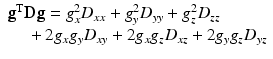
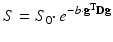
where g T is the transpose of g. The right side of the equation simply shows what you would obtain if you did the symbolic math by hand using the vector and tensor element symbols from Eq. (4.5). The outcome of this expression—if we were to fill in some specific numbers representing the vector and tensor elements—is thus a single scalar number: the value of our tensor model, along a given direction. As we will now employ such a tensor to symbolize the ADC values, we can simply plug it into the good old Stejskal-Tanner Eq. (4.1) to obtain the following expression :
(4.5)
(4.6)