Functional AFM Imaging of Cellular Membranes Using Functionalized Tips

Fig. 1.

AFM tip functionalization with Fc fragments via NHS–PEG–Aldehyde linker. (i) Aminofunctionalization of silicon nitride (Si₃N₄) AFM tips via silanization with 3-aminopropyltriethoxysilane (APTES) in gas phase. (ii) Use of heterobifunctional NHS–PEG–Aldehyde linker for the flexible attachment of underivatized protein onto the AFM tip. (iii) A ligand molecule is coupled to another free functional end of PEG-linker. The C=N double bond is usually fixed by a reaction with sodium cyanoborohydride (NaCNBH₃).

Clean AFM cantilevers in chloroform for 10 min and dry with a gentle nitrogen stream. Amino (–NH₂) groups are produced on the AFM tips by gas phase silanization with 3-aminopropyltriethoxysilane (APTES) (23). First, APTES is freshly distilled under vacuum. Flood a desiccator (5 L) with argon gas to remove air and moisture. Then place two small plastic trays (e.g., the lids of Eppendorf reaction vials) inside the desiccator, with 30 μL of APTES and 10 μL of triethylamine (see Note 7) separately pipetted into the two trays. Place pre-cleaned AFM cantilevers nearby on a clean inert surface (e.g., Teflon) within the dessicator, and close the dessicator. After 2 h of incubation, remove the trays with APTES and triethylamine. Again, flood the desiccator with argon gas for 5 min. Leave the tips inside for 2 days in order to “cure” the APTES coating.

For the attachment of the PEG linker, dissolve 3.3 mg of NHS–PEG₂₇–Aldehyde in 0.5 mL of chloroform and transfer with a glass pipette to a small glass reaction chamber.

Add 30 μL of triethylamine and carefully immerse the cantilevers in this solution for 2 h at RT. Cover the reaction chamber with an upside-down beaker to avoid chloroform evaporation (see Note 8).

Then wash cantilevers extensively (3×) in chloroform, dry with a gentle nitrogen stream and put in a clean dry petri dish, which is then covered with Parafilm. Arrange cantilevers in a circular manner so that the tips are found in the center direction.

For ligand coupling, mix a 50 μL aliquot of Fc fragment stock solution (∼1 mg/mL in PBS, freshly thawed from −25 °C) with 150 μL of 1× PBS. Pipette the protein solution onto the cantilevers as a small drop to cover all tips with the liquid.

Immediately add 2 μL of 1 M NaCNBH₃ (freshly prepared each time) and mix carefully with a pipette. Allow the reaction to be carried out for 1–2 h.

To inactivate free aldehyde groups on the tips, add 5 μL of 1 M ethanolamine hydrochloride (pH 9.6 pre-adjusted with NaOH and stored in aliquots at −25 °C) for 10 min.

Finally, wash the cantilevers with 1× PBS (AFM working buffer) (3×) and store at 4 °C until used (see Note 9).

3.2 Cell Preparation for AFM Measurements

Wash glass slides with 70% isopropanol or ethanol and subsequently with distilled water or 1× PBS, put the glass slides in petri dishes. If any liquid drops remain on the slides, pump them carefully away.

Cells are grown on the glass slides. When the cells achieve the desired confluence state (∼50%), they are “gently” fixed with 4% PFA (16). Warm an aliquot of 4% PFA fixative, pump away growth media, wash the cells with HBSS (1×), incubate in pre-warmed 4% PFA for 30–60 min at 37 °C, and then wash (3×) the fixed cells with HBSS containing Ca²⁺. The fixed cells can either be immediately used for AFM measurements or stored at 4 °C for several days (see Note 10).

3.3 Functional AFM Imaging on Cell Membranes

Connect the PicoTREC box to the head electronics, MAC box, and AFM controller according to the PicoTREC user manual.

Turn on the AFM controller, MAC box, computer, lamps, and other major electronics and allow to warm up for at least 30 min in order to minimize the drift of electrical signals during the experiment.

Use the stepper motor to move the sample plate, ensuring that there is enough distance (1.5–2 mm) between the sample plate and AFM scanner. This will prevent a sudden breakage of the AFM cantilever during the further montage.

Prior to mounting the cell probe, place some reflective material, such as a gold-coated mica or aluminum sheet, onto the sample plate and cover it with a mica sheet. Mount the glass slide with fixed cells on the sample plate, carefully fix the liquid cell with two clips on the glass slide and fill it immediately with ∼600 μL HBSS with Ca²⁺. Take care that the cells do not dry out. Finally, mount the sample plate with the cell probe in the AFM.

Carefully mount the functionalized AFM cantilever on the AFM scanner, taking care that the cantilever does not dry out.

Orient the scanner, mount it onto the microscope stage, fix, and plug it in. Check with the CCD camera that the cantilever has not broken during the scanner mounting. If any air bubbles are observed, remove the scanner, carefully blot dry with the corner of a piece of filter paper, and then repeat this step again.

Set up the instrument for MAC Mode.

Ensure that the TREC servo on the front of the PicoTREC box is in the OFF position.

Choose an appropriate calibration file for the AFM scanner.

10.

Set one image channel to “Topography” (both in trace and retrace direction) and a second channel to “Aux In BNC” (both in trace and retrace direction) (see Note 11).

11.

Perform a frequency sweep by tuning the functionalized MAC Lever far away from the sample surface (∼60 μm) (Fig. 2), and choose and set the starting drive amplitude (the amplitude meter on the MAC box should read ∼6 V (MAC1.2 box) or ∼1.5–2 V (MACIII box)) (see Note 12). As a rule of thumb we choose the excitation frequency 20% lower than the resonance frequency at large distances (resulting in ∼8 kHz excitation frequency, indicated by an arrow in Fig. 2).

Fig. 2.

Typical amplitude–frequency (resonance or tuning) curve acquired in buffer (HBSS) with a MAC Lever. Tuning curves are recorded by varying the excitation frequency from 5 to 20 kHz; tip-sample separation distance is 60 μm. A distinct resonance peak is obtained at ∼10 kHz (using a cantilever with a nominal spring constant of 0.15 N/m). A frequency of ∼8 kHz is used as excitation frequency for imaging (indicated by an arrow).

12.

Perform a rough approach to the surface. Withdraw the tip and place the tip over a cell of interest with the help of the CCD camera. Adjust the drive signal to typically attain either ∼6 V on the MAC1.2 box or ∼1.5–2 V on the MACIII box.

13.

Approach the sample surface and begin imaging a whole cell (typically at a scan size of ∼60 × 60 μm²). Consequently reduce the scanning area to ∼2 × 2 μm² by choosing relatively flat cell surface (Fig. 3 left). Use a maximum lateral scan speed of ∼3 μm/s; this will result in a total recording time of ∼12 min per image (with a resolution of 512 lines per image). Scan using gain settings as high as possible, but without producing excessive noise. Start with a very low imaging force (high amplitude set-point so that the tip slightly touches the surface; one can check this by opening the “real time cross-section” window and follow the topography cross section in trace and retrace) and, consequently, reduce the amplitude set-point to get a fairly good overlay of trace and retrace cross-section lines. Avoid reducing the set-point further; this can result in strong cross talk of topography information into the recognition image (24). Setting the proper imaging amplitude is critical (24): it must be large enough to stretch the PEG linker, slightly deflect the cantilever as it oscillates over the target molecule, and detect the binding interactions. Nevertheless, the oscillation amplitude should remain small enough so that the binding does not rupture on each oscillation. Therefore, an imaging amplitude of ∼8–15 nm (this typically corresponds to ∼1.5–2.5 V on the amplitude meter of the MAC1.2 box) is recommended for TREC imaging (see Subheading 3.4 below to determine the free oscillation amplitude in nm). Generally, the proper amplitude regime for the observation of recognition events differs from one functionalized cantilever to another, depending upon the length of the linker molecule, on the exact location of the linker molecule on the tip apex, and the size of the attached molecule. Therefore, actual settings will vary, and you might have to change the drive amplitude and approach again.

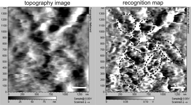
Fig. 3.

Simultaneously recorded Topography (left ) and RECognition (right ) images on J774.A1 cells with a Fc functionalized tip. Recognition map of Fcγ receptor domains (black spots embedded by black circles) represents an amplitude reduction due to specific binding between Fc molecules on the AFM tip and FcγRs on the cell surface. Scale bars are 250 nm.

14.

Recognition is observed as dark “hot” spots in the “Aux in BNC” image channel (Fig. 3 right). Normally the recognition maps remain unchanged during 1 h of continuous scanning. If no recognition signal is visible after adjusting the gains and amplitude after several image frames, the functionalized MAC Lever must be replaced. We suggest preparing as many functionalized MAC Levers as possible (a minimum of 5) to ensure at least one “good” MAC Lever is available for TREC imaging.

15.

Perform the blocking experiment (see Note 13). Inject Fc fragments at high concentration (∼0.8 mg/mL) very slowly and gently into the fluid cell while scanning the cell surface. The first scan after injection might not demonstrate immediate changes in the recognition map. After 2–3 scans, one can observe subsequent disappearance of dark spots with imaging time as the free Fc fragments will bind to Fcγ receptors on the macrophage surface (16) (see Note 14). After blocking experiments, simultaneously recorded topography images should remain unchanged—indicating that the blocking does not affect membrane topography.

Only gold members can continue reading. Log In or Register to continue