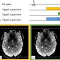
Laura Adela HARSAN1, Laetitia DEGIORGIS1, Marion SOURTY1, Éléna CHABRAN1 and Denis LE BIHAN2 1 ICUBE, CNRS, Université de Strasbourg, France 2 NeuroSpin, CEA, Gif-sur-Yvette, France A century before the first functional MRI scans, Roy and Sherrington (1890) wrote: We conclude then, that the chemical products of cerebral metabolism contained in the lymph which bathes the walls of the arterioles of the brain can cause variations of the caliber of the cerebral vessels: that in this re-action the brain possesses an intrinsic mechanism by which its vascular supply can be varied locally in correspondence with local variations of functional activity. The authors were thus already describing a mechanism that would later be called neurovascular coupling (NVC). This phenomenon is the foundation of hemodynamic imaging techniques, such as blood oxygenation level dependent (BOLD) functional magnetic resonance imaging, or BOLD-contrast fMRI, which detects the cerebral activity related to a task or, more recently, the synchronous activity of neural networks at rest. The first part of this chapter presents the basics of the BOLD signal’s origin and describes how the variations of this signal are related to transient changes in neuronal activity. Subsequently, we present the principles of functional connectivity mapping based on resting state fMRI data modeling and examples of clinical applications and translational animal studies. Functional MRI data pre-processing and subsequent statistical analysis is very complex and will not be described in this chapter. BOLD-contrast functional MRI is an indirect method to produce images of cerebral activity based on the detection of local variations in blood flow and oxygenation induced by neuronal activity (Ogawa et al. 1990). This technique links (1) the paramagnetic nature of deoxyhemoglobin (DHb), modifying the magnetic susceptibility of blood and causing a change in T2*, with (2) the NVC based on the dynamic relationship between cerebral metabolism, cerebral blood flow (CBF), cerebral blood volume (CBV) and neuronal activity. NVC depends on the vasoreactivity of the cerebrovascular system. Red blood cells transport oxygen via hemoglobin, gathering oxygen in the pulmonary circulation system and offloading it in the capillaries to meet the tissue needs (Figure 5.1(a)). Therefore, hemoglobin circulates in the blood in two states: an oxygenated state (OHb) and a deoxygenated one (DHb). Figure 5.1. Cerebral blood circulation. (a) Coronal slice of a mouse brain acquired with a multiphotonic microscope, showing the arteries in red and the veins in blue (modified with permission from Kirst et al. 2020). (b) Percentage of OHb and DHb in cerebral blood vessels These changes lead to a modification of the oxygen saturation (SO2) in the blood, which is a measure of the OHb percentage. Arterial blood is oxygenated at 100%, but exchanges in the capillary network reduce the oxygen saturation level in the venous blood to levels that vary overall between 70% and 60% (Figure 5.1(b)) depending on the region. In 1936, Linus Pauling (Nobel prize in Chemistry in 1954) and Charles Coryell demonstrated that the hemoglobin molecule has different magnetic properties depending on its state of association with oxygen (Pauling and Coryell 1936; Figure 5.2). On the one hand, OHb is diamagnetic, showing no unpaired electrons and a magnetic moment equal to zero. On the other hand, DHb is paramagnetic with two unpaired electrons and a non-zero magnetic moment. When located within a static magnetic field, DHb causes a local perturbation of the magnetic field. This induces changes in magnetic susceptibility, leading to the production of magnetic field gradients in intravascular and perivascular spaces. The non-uniform field around vessels leads to a decrease in the relaxation time T2* and therefore reduces the MRI signal intensity. Thus, DHb is an authentic endogenous contrast agent. Later, Ogawa et al. performed an in vivo study at 7 T in anesthetized rats, hypothesizing that modifications of the blood oxygen proportion would affect the detectability of cerebral blood vessels on T2*-weighted images. The authors showed that the cortical surface had a uniform texture when the rats were breathing pure oxygen (Figure 5.2(a), right), while a 21% decrease in oxygen – that is, while rats were breathing normal air – led to regions with a signal loss in areas matching blood vessel locations (Figure 5.2(b), right). Since cerebral metabolic processes require oxygen provided through blood circulation, Ogawa suggested using this contrast, called blood oxygenation level dependent (BOLD), as an indirect measure of changes in cerebral activity (see Kim and Ogawa 2012; Huettel et al. 2014). Figure 5.2. Magnetic properties of oxyhemoglobin (OHb-A) and deoxyhemoglobin (DHb-B) COMMENT ON FIGURE 5.2.– (a) Diamagnetic properties of OHb. On the right, a schematic illustration of a coronal slice in the brain of a rat breathing pure oxygen, with a uniform cortical surface. (b) Paramagnetic properties of DHb. Deoxygenated blood locally perturbs the magnetic field B0. The coronal slice shows the blood vessels (loss of signal in black – in T2* weighting) after inhaling air, correlated to an increased DHb concentration. Figure adapted from Ogawa et al. (1990). The physiological foundations behind BOLD fMRI are complex. Here, we present a summary of this topic and highlight excellent literature reviews (Kim and Ogawa 2012; Huettel et al. 2014; Howarth et al. 2021). At rest, the cerebral metabolic rates of O2 (CMRO2: ~5 mL/min/100 g) and glucose (CMRglu: ~ 31 μmol/min/100 g) represent 20% and 25%, respectively, of the total consumption of our bodies (Ter-Minassian 2006). The blood flow is also very high in the entire brain, with some variations depending on cerebral areas, and constitutes 20% of the cardiac flow at rest. This resting energy metabolism is mainly related to synaptic activity (Shulman et al. 2004), and thus to intercellular communication. To satisfy these high metabolic needs, the brain has access to only one source of energy – the glucose delivered through blood circulation. Astrocytes (glial cells in brain tissue) have been reported to play a major role in cerebral metabolism by regulating the microcirculation and the distribution of energetic substrates according to neuronal activity (Magistretti 2011). However, 80% of the glucose consumption is related to synaptic activity at rest. Therefore, the resting state, conceptualized by the American neurologist Marcus Raichle as a “default mode” (Raichle et al. 2001), is a particularly energy-consuming activity. The neuronal activity increase following a stimulation (Figure 5.3), a cognitive task or activity, leads to local synaptic and electrical responses, increasing the tissue’s energy needs. In that case, a fast metabolic response occurs, increasing the glucose (CMRglu between 20 and 40%) and oxygen consumption (CMRO2 between ~5% and 20%) (Figure 5.3c(1)). Figure 5.3. Physiological principle of BOLD fMRI COMMENT ON FIGURE 5.3.– (a) In basal conditions (before stimulation), the arteries are 100% oxygen-saturated, compared to about 60% saturation in the veins. O2 is exchanged at the capillaries. (b) Cerebral activation due to a stimulus produces (c) a rapid local metabolic and vascular response with increased consumption of glucose (CMRglu) and oxygen (CMRO2), as well as an increased cerebral blood flow (CBF) and cerebral blood volume (CBV). The local O2 supply exceeds the exchanges in capillaries, leading to an excess of OHb in the venules and an increased OHb/DHb ratio. This translates into decreased magnetic susceptibility effects and a small increase in BOLD fMRI signal. Vasoactive signals are sent to surroundings of arterioles and capillaries, thereby dilatating the upstream arterial vessels. A hemodynamic response occurs 1–2 s after a stimulation, inducing an increase in the regional cerebral blood flow (rCBF) by 30–70% of the CBF by 5–30%. According to the so-called Balloon model (Buxton et al. 1998), an arteriole vasodilation and an increased CBF lead to a passive vasodilation of venules and veins thanks to their elasticity. While the increased rCBF addresses the higher needs in glucose in the active region, the local oxygen supply exceeds the more moderate increase in its extraction at the capillaries. Therefore, the oxygenation rate in veinous blood changes, showing higher oxyhemoglobin (diamagnetic) in venous capillaries of the activated area relatively to the DHb (paramagnetic) concentration (Figure 5.3c(2)). The signal increase reaches a peak 5–7 s after the beginning of a stimulation, a cognitive task or activity. The maximum amplitude is maintained for the duration of the activation time. Once the activation phase ends, blood flow and volume decrease, which translates into a gradual return of the signal intensity to the basal level. Since the intensity of the BOLD effect depends on the static magnetic field B0, the observed signal variations are between 1 and 5% for a 1.5 T magnetic field, while they are greater than 20% at a 4 T field (Turner et al. 1993). The dynamic of the neurovascular system making the link between stimuli and measured BOLD signals is characterized by the hemodynamic response function (HRF, Figure 5.4). The hemodynamic response induced by a short stimulation (Figure 5.4(a)) can be decomposed into several phases related to NVC: (1) an initial decrease in the signal at least 2 s after the stimulation (known as “initial dip”) related to an immediate oxygen extraction that precedes the blood flow increase; (2) a much greater increase in the amplitude of the signal from 5 to 7 s after the stimulation; (3) a signal undershoot below its basal level before stabilizing within about 20 s. Therefore, there is a time delay between the cerebral activation and the detection of the peak signal in BOLD fMRI. The maximum amplitude of the hemodynamic response will be maintained depending on the duration of the stimulation (Figure 5.4(b)). Figure 5.4. Theoretical representation of the hemodynamic response following a short stimulus (a) and sustained stimulation (b) Several electrophysiological methods have been combined with BOLD fMRI to test the relationship between neuronal activity and BOLD signal in a more direct way (Logothetis and Wandell 2004). Using electrical recordings of the visual cortex of anesthetized monkeys, Logothetis and Wandell showed that the BOLD signal would be much more correlated with the local field potentials (LFPs) than with multi-unit activity (MUA) of the axons. The authors concluded that the BOLD signal mainly reflects electrical inputs and their intracortical processing rather than output discharges. However, in some regions, multi-unit neuronal discharges are only temporary, while the LFP is sustained, suggesting a more linear relationship between the BOLD signal and the local potential. In rodents, neuronal activity can be controlled using optogenetic approaches (Deisseroth 2011) while recording the BOLD signal via MRI (Kahn et al. 2011). Kahn et al. used an optogenetic stimulation to induce a BOLD MRI signal that accurately reflected the imposed neuronal discharges and showed an excellent linearity (Kahn et al. 2011). Despite these breakthroughs, understanding the cerebral activity mechanisms underlying the BOLD signal remains a very active research topic (Schwalm et al. 2017). The recent combination of calcium imaging (measuring the variations in intraneuronal and/or intra-astrocyte calcium concentration as a marker of cellular activity) with BOLD fMRI in preclinical studies (Pradier et al. 2021) offers new ways of studying the direct relationship between brain cell activity, the physiological response following the activity of these cells and the detected fMRI signal. Thus, the association between neuronal activity and BOLD signal is indirect. Moreover, it is modulated by a great number of parameters such as the quality and intensity of neuronal response to a stimulus, the NVC, the intrinsic features of the hemodynamic response in the different brain regions, as well as the hardware parameters of fMRI acquisitions. Several methodological aspects must be considered to detect the BOLD effect in MRI with good sensitivity and specificity associated with neuronal activity. Sensitivity is described as the capability of BOLD fMRI to reveal brain activity with an increase in neuronal activity. It is defined by hardware characteristics, such as magnetic field intensity, voxel size, bandwidth, sequences, echo time (TE) or spatial encoding. Specificity describes the ability to properly localize signals related to neuronal activity changes. This specificity is disturbed by the higher sensitivity of the BOLD signal to the venous drainage network compared to the neurons. In fact, the BOLD signal is divided into two components: an intravascular component related to T2* variations in the vessels and an extravascular component originating from perivascular tissue in contact with the activated neurons. Thus, increasing the fMRI specificity means being able to better discriminate between the intravascular and extravascular components of the BOLD signal, and therefore detection of activations closer to the recruited neurons (Uludağ et al. 2009). The BOLD effect causes variations of T2* (∆R2*, R2* = 1/T2*). This requires the use of ∆R2* sensitive sequences, that is, T2* weighted, the premium choice being gradient echo (GE) sequences. Using such sequences, the first fMRI studies in humans (Menon et al. 1993) found a link between the echo time (TE) and the sensitivity to detect BOLD signal variations following a stimulation (here, a photic stimulation). If S is the signal intensity in a voxel of an image obtained at an echo time TE, then the percentage of BOLD signal change (ΔS/S) after stimulation can be calculated using the following approximation (Menon et al. 1993; Uludağ and Blinder 2018): In this formula, S0 represents the intrinsic MRI signal at TE = 0. By deriving the expression, the BOLD signal can be estimated as: The BOLD signal change (ΔS/S) in percent can thus be estimated as: showing a direct dependency with TE value. To model this relationship in a more accurate way, the effects of different tissue behaviors (extravascular, intravascular) must be considered (Havlicek et al. 2017). Gradient-echo echo-planar imaging (GE-EPI) is the standard approach for BOLD fMRI scans. In conventional GE-EPI protocols, the signal is measured for a single TE, specifically chosen to match the mean T2* of the tissue and maximize the sensitivity. However, T2* values vary a lot across brain areas and tissues and depend on the intensity of the magnetic field (Cheng et al. 2015). Using multi-echo (ME) scan protocols, BOLD-contrast sensitivity can be optimized through weighting schemes that combine fMRI signals of different TEs (Posse 2012). The optimization of TE can also improve spatial specificity: since the T2* of the venous system is quite shorter than the T2* in tissues, the extravascular BOLD signal component can be emphasized using a higher TE. The combination of ME sequences with multiband (MB) techniques provides a way of obtaining high temporal and/or spatial resolution images (Cohen et al. 2021). Spatial resolution refers to the ability to distinguish changes in images across different spatial locations, while temporal resolution refers to the ability to distinguish activity changes at a given location over time. Spatial resolution is closely related to spatial activation specificity. In conventional GE-EPI protocols, spatial resolution is about a few millimeters (2–3 mm). High magnetic fields (3T and above) are without a doubt of great benefit for fMRI as they provide better spatial imaging resolution, higher BOLD contrast sensitivity and better microvascular specificity. High-field applications demonstrate the feasibility of very accurate functional mapping (Figure 5.5; Yang et al. 2021) when BOLD fMRI is compared to alternative fMRI techniques, such as those based on CBV mapping (Huber et al. 2021). Figure 5.5. Mapping of cerebral activity within various neuronal layers of the motor cortex following activation of alternated movements of the right thumb and index. (a) Activation detected via BOLD fMRI (GE-EPI) at 7 T. (b) Mapping of cerebral blood volume via a VASO (vascular space occupancy) sequence. Figure modified with permission from Yang et al. (2021) Temporal resolution in fMRI relies on the acquisition of repeated measures over time for each voxel to explore the brain function. In such contexts, echo-planar acquisitions are fast and cover the entire brain (a volume of images) in only 2–3 s. Each image is acquired in 20–150 ms depending on the sequence parameters and the employed hardware. fMRI signals are thus usually described as “time-courses”. Decreasing the repetition time (TR) for a better sampling of the hemodynamic fMRI response is beneficial as it improves the estimation of the response. Thanks to important technical advancements, higher temporal resolutions have been recently achieved. For example, the MB (Demetriou et al. 2018) and simultaneous multislice (SMS) (Bhandari et al. 2020) acquisitions decrease TR (from 2 s to 300 ms). Experimental design is a key point in activation fMRI studies and the timeline of the stimulation paradigm is fundamental as it has to be synchronized with the image acquisition. A paradigm design consists of a temporal sequence of stimuli received and/or tasks performed by the subject, whose goal is to trigger the cerebral activity of interest. fMRI does not allow for quantification of the level of cerebral activity in absolute terms; it detects the difference in cerebral activity during the execution of the chosen task with respect to a reference state (at rest or while performing another task). The alternation of the different conditions defines the type of paradigm design. “Block” paradigms consist of a successive stimulus train (or block) of a few tens of seconds during which stimuli occur repeatedly at regular intervals. In event-related paradigms, short-duration stimuli are induced individually in a pseudo-random time sequence to prevent anticipation effects from the participant. Whatever the paradigm design implemented, the delay between the neuronal activation and the measured hemodynamic response is taken into account. Theoretical curves of the hemodynamic response can be established and then modeled to perform statistical analyses to identify voxels whose signal variation is related to the paradigm. Animal imaging studies (Gil et al. 2021) have demonstrated their importance for the better understanding of the physiological (NVC) or pathological aspects of the cerebral response following a stimulation or regarding questions about the specificity of the BOLD signal at very high fields (Jung et al. 2021). The use of magnetic fields higher than 7 T is now common in preclinical imaging studies in rodents. Using a sequence with high spatial and temporal resolutions at 15.2 T in anesthetized mice, Jung et al. (2021) have recently shown that the detection timeline of the first BOLD responses (from one active cerebral area to another) reflects the direction of neuronal information flow (Figure 5.6). In fact, sensory stimulation in mice (electrical stimulus of the left paw) using a block paradigm produces a sequence of fast activations of thalamic nuclei, sensorial cortex and motor cortex. This coincides with the known sequence of neural activation. fMRI studies involve several image pre-processing steps that are fundamental for further statistical group analyses. Data processing fMRI pipelines can vary depending on the type of acquisition and target analysis. These analyses are not within the scope of this chapter, but they are nevertheless important for interpreting the results. Figure 5.6. Block paradigms for fMRI stimulation in mice, using an electrical stimulus of the left paw and corresponding functional maps of the BOLD response. The timeline of the first detected BOLD responses is the following: (1) thalamus (TH), (2) somatosensory cortex (SS) and (3) motor cortex (MO). Figure modified with permission from Jung et al. (2020) The large-scale organization of cerebral functioning is based on two fundamental principles: segregation and integration of information (Park and Friston 2013). Functional segregation refers to the existence of brain regions specialized in a given function. However, these brain areas do not work in an isolated way among each other: they are defined as nodes that interact in a coherent and dynamic way to process information, giving rise to the concept of functional integration (Varela et al. 2001). Due to the interaction between cerebral regions, the brain can be studied as a network, leading to the notion of connectivity. A brain structure supporting a given function can thus be considered as a set of specialized cortical areas linked by functional integration (Friston 2005). Therefore, functional specialization and integration are not mutually exclusive but rather complementary and are mediated via cerebral “connectivity”, a fundamental notion in neuroscience (Park and Friston 2013). In this context, three types of cerebral connectivities are considered: (i) structural connectivity (SC), mapped using diffusion tensor MRI (DTI) and tractography and allowing anatomical connectivity to be studied through the analysis of white matter fibers; (ii) functional connectivity (FC), studied via resting-state fMRI based on the analysis of the statistical correlations between time courses of the BOLD signal in different brain regions; (iii) effective connectivity (EC), for investigating the direct influence of one brain region to another. Here, causal interactions related to a task or information flows are studied and described by dynamic causal models. Resting-state fMRI (rs-fMRI) maps the intrinsic cerebral activity to identify its functional networks. In such acquisitions in humans, subjects are scanned “at rest” and asked to relax, not think about anything in particular, close their eyes or focus on a specific point in their field of view for the entire scan.
5
Functional MRI
5.1. BOLD-contrast functional imaging and brain connectivity
5.1.1. Introduction
5.1.2. BOLD-contrast functional MRI principles
5.1.2.1. Cerebral circulation

5.1.2.2. Paramagnetic properties of DHb

5.1.2.3. Physiology of neurovascular response
5.1.2.3.1. Resting brain metabolism
5.1.2.3.2. Neurovascular coupling

5.1.2.3.3. Hemodynamic response function

5.1.2.3.4. What kind of neuronal activity for BOLD fMRI signal?
5.1.2.4. BOLD signal detection
5.1.2.5. BOLD fMRI acquisition methods and sequences


5.1.2.5.1. Spatial and temporal resolution in fMRI

5.1.3. fMRI activation paradigms
5.1.3.1. fMRI with stimulation paradigms in preclinical studies

5.1.4. Resting fMRI and functional cerebral connectivity mapping
5.1.4.1. Observing and modeling the brain as a large-scale network
5.1.4.2. Resting fMRI and functional cerebral connectivity mapping
Related posts:
Stay updated, free articles. Join our Telegram channel

Full access? Get Clinical Tree


