Groupwise Multi-scale Parcellation of the Cortex

vertices, and assume all surfaces to be registered to the same reference [9]. As a result, all surface vertices have direct correspondence across all subjects. Furthermore, we consider that a $N_v \times N_v$ tractography matrix $\chi _{S_i}$ has been computed from diffusion data for each subject . Each row of this matrix $\chi _{S_i}(\mathbf {v})$ describes how a vertex $\mathbf {v}$ is connected to the rest of the cortical surface.

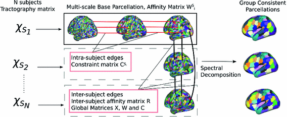
The proposed method is illustrated in Fig 1. For each subject, a set of high resolution parcellations is constructed for L different resolution layers (base parcellation). These parcellation layers then serve as the basis of a multi-scale groupwise spectral clustering problem, where the affinity between vertices is described by the tractography matrix, and edges across resolutions and subjects force the parcellations to be consistent.

Fig. 1.

Illustration of the proposed method. Each subject $$S_i$$

is associated with a connectivity matrix $\chi _{S_i}$ that drives the construction of a multi-scale base parcellation. Intra-subject edges (between base parcellation resolutions) and inter-subject edges (between all pairs of subjects at the coarsest parcellation resolution) are built to allow a common spectral decomposition of the affinity matrix (connectivity profiles correlation).

2.1 Base Parcellation

The first step towards building our groupwise parcellation is to capture structural connectivity information at multiple scales through the construction of supervertices at different resolutions. Similarly to superpixels [1], supervertices can be seen as an initial over-segmentation of the cortical surface based on connectivity information such that vertices within a supervertex have very similar connectivity profiles. We rely on the geodesic distance between vertices to obtain spatially contiguous supervertices, while the correlation between their connectivity profiles enforces homogeneous connectivity.

We are inspired by the method proposed in [14] that relies on Fast Marching to compute geodesic distances for surface segmentation. In this setting, the computation of the geodesic distance $d(\mathbf {v_0},\mathbf {v})= U(\mathbf {v})$ from vertex $\mathbf {v_0}$ can be reformulated as a front propagation problem, where U follows the Eikonal equation $\Vert \nabla U \Vert F=1$ which can be solved using the Fast Marching algorithm. F is the speed function characterising the front propagation. We can compute a correlation dependent geodesic distance by defining a correlation weighted speed function: $F(\mathbf {v})= \exp \left( \mu \rho (\chi _{S_i}(\mathbf {v_0}),\chi _{S_i}(\mathbf {v}))\right)$ . Here, $\rho (.,.)$ is the Pearson’s correlation coefficient between the vertices’ connectivity profiles $\chi _{S_i}(\mathbf {v})$ and $\mu$ is a weighting parameter. In this setting, the front will propagate faster towards vertices that have a high correlation (i.e. similar connectivity profiles) with the source vertex $\mathbf {v_0}$ .

Each supervertex resolution is computed through an iterative approach. Given a specified number of

supervertices, we initialise by uniformly sampling

seeds across the brain’s cortical surface. At each iteration, we first compute the correlation weighted geodesic distance from each seed to the rest of the surface, and build supervertices by assigning a vertex to its closest seed. We then reevaluate the seeds by selecting, for each supervertex, the vertex that has the highest correlation with the rest of the cluster. This process is iterated until convergence for the L different levels.

Each base parcellation level is associated to a $N_l \times N_l$ merged connectivity matrix, constructed by adding the fibre counts across vertices. The level’s affinity matrix

is defined as the Pearson’s correlation coefficient between those merged connectivity profiles. In order to obtain spatially contiguous parcels, correlation weighted edges are only constructed between supervertices that are adjacent.

Our next step is to build connections between the different base parcellation levels, so as to recover a common partition of the cortical surface across resolutions.

2.2 Intra-subject Connections Between Resolutions

We seek coherence across resolutions by enforcing supervertices that are in similar locations on the cortical surface to be assigned to the same parcels through the construction of inter-resolutions edges.

For a given resolution level l, each supervertex is connected to a supervertex at the finer level

if they share vertices on the original cortical surface. The strength of the edge is defined by the amount of overlapping vertices, so that the same parcellation result is imposed on supervertices that are the most similar. The intra-subject, inter-resolutions links can be written as:

$\begin{aligned} C_{l-1,l}(j,k) = \frac{\vert s_l^j \cap s_{l-1}^k \vert }{\vert s_l^j \vert } \end{aligned}$

(1)

where

is the set of vertices at the original resolution that belong to the j-th supervertex at resolution level l and $\vert s_l^j \vert$ is the number of vertices in

In this setting, we can estimate a parcellation for a single subject

that is consistent across resolutions using the multi-scale normalised cut approach [19]. For each level l, we aim at finding a K-way parcellation matrix $X_l \in \{0,1\}^{N_v \times K}$ defined as:

$\begin{aligned} X_l (i,j)= {\left\{ \begin{array}{ll} 1 &{} \text {if }s_l^i\ \in \ \text {parcel j} \\ 0 &{} \text {otherwise} \end{array}\right. } \end{aligned}$

(2)

The multi-scale parcellation and affinity matrices can then be constructed as follows:

$\begin{aligned} X^{S_i}= \left( \begin{array}{c} X_1 \\ \vdots \\ X_L \end{array} \right) \!\! , W^{S_i}= \left( \begin{array}{ccc} W_1 &{} &{} 0\\ &{}\ddots &{}\\ 0&{} &{}W_L \end{array} \right) \end{aligned}$

(3)

Finally, we build a constraint matrix that encodes the inter-resolution links and ensures consistency of the recovered parcellation across resolutions:

$\begin{aligned} C^{S_i}= \left( \begin{array}{cccc} C_{1,2} &{} -I_{N_2} &{} &{} 0\\ &{}\ddots &{} \ddots &{}\\ 0&{} &{}C_{L-1,L} &{} -I_{N_L} \end{array} \right) \end{aligned}$

(4)

Here, $I_{N_l}$ is the $N_l \times N_l$ identity matrix and

is the number of supervertices at scale l. This matrix forces the obtained parcellation to be consistent across scales through the following constraint equation:

$\begin{aligned} CX=0 \end{aligned}$

(5)

Optimisation of the multi-scale normalised cut criterion, subject to the inter-resolution constraint [19], yields a single subject parcellation that captures local connectivity information at different scales. Comparing the obtained parcellations within a group is however a very challenging task as there are no direct matches between parcels, and anatomical variability (as well as registration errors) can cause different subjects to have very different parcel boundaries. This issue can be addressed by performing a concurrent parcellation of all the subjects within the group to directly obtain correspondences between parcels.

2.3 Inter-subject Connections

Spectral clustering offers the possibility to integrate different subjects in the same framework in a very natural manner. A group consistent parcellation can be obtained through a joint estimation of the parcellation matrix X across subjects. The groupwise parcellation, affinity and constraint matrices are defined as:

$\begin{aligned} X= \left( \begin{array}{c} X^{S_1} \\ \vdots \\ X^{S_{N}} \end{array} \right) \!\! , W= \left( \begin{array}{ccc} W^{S_1} &{} &{} R\\ &{}\ddots &{}\\ R^T&{} &{}W^{S_{N}} \end{array} \right) \!\! , C= \left( \begin{array}{ccc} C^{S_1} &{} &{} 0\\ &{}\ddots &{}\\ 0&{} &{}C^{S_{N}} \end{array} \right) \end{aligned}$

(6)

Matching parcellations are enforced by adding inter-subject connections encoded in the matrix R. Following [12], we only connect the coarsest resolution layers. This step is essential in our case as it relaxes the need for a precise registration in addition to allowing individual differences at the highest resolution.

Let us consider that all subjects have been registered to a common surface mesh. Similarly to the multi-scale parcellation approach, we seek a common parcellation across subjects by forcing supervertices in similar locations to belong to the same parcel. To this end, a supervertex from subject i is connected to a supervertex from subject j if they share the highest amount of overlapping surface vertices and have the strongest correlated connectivity profiles. We define the inter-subject edges between matching supervertices as follows:

$\begin{aligned} R(s^i(S_1),s^j(S_2)) = \alpha \rho (s^i(S_1),s^j(S_2)) \end{aligned}$