Hierarchical Cluster Analysis to Aid Diagnostic Image Data Visualization of MS and Other Medical Imaging Modalities

Fig. 1

Tumor tissue embedded in a gelatin block and four markers placed in four corners

MRI images were acquired using the 0.25 T Esaote GScan. The sample was centrally placed with a dedicated wrist coil and a range of sequences performed FOV (160 × 160). Optimal results were achieved from the T2-weighted Gradient Echo (3NEX) and XBone (4NEX) sequences; 2 mm slices (see Notes 1 and 2 ) (Fig. 2).

Fig. 2

T2-weighted MRI image of the tissue specimen

The tissue sample was frozen and then cryosectioned prior to MALDI MSI data capture.

Peptide mass fingerprints and MALDI Images were performed using the Applied Biosystems Qstar Pulsar i.

2.2 X-Ray Mammogram Image Data

Anonymized X-ray mammogram image data were acquired as part of a screening program using Full Field Digital Mammography (FFDM) system with the pixel spacing of 70 μm (0.070 mm) (see Note 3 ). The approximate location and extent of abnormalities were marked by an expert radiologist (Fig. 3).

Fig. 3

X-ray mammogram image with the location and size of the abnormality marked by the expert

2.3 mpMRI Image Data

Anonymized MRI image data were acquired as part of diagnostic investigation. The images were acquired with pixel spacing of 1000 μm (1.0 mm) and 1.0 mm spacing between slices. The multi-parametric images were acquired as T2-weighted before injecting intravenous contrast (Fig. 4) and T1-weighted Dynamic Contrast Enhanced (DCE) images. In T2-weighted images, with a small “Field Of View” (FOV), tumour will appear as signal loss (dark).

Fig. 4

T2-weighted MRI image section of the prostate

The DCE MRI images are acquired after intravenously injecting gadolinium chelate contrast (Fig. 5). After injecting intravenous contrast the temporal sections were acquired 16 times at an interval of approximately 10.49 s. Figure 6 lists the Prostate part of the section acquired from time 10:23:51.6275 (SER26) to time 10:26:33.9775 (SER11) (Fig. 6).

Fig. 5

Dynamic Contrast Enhanced MRI image section of the Prostate post contrast injection

Fig. 6

Temporal sequence of the DCE MRI image of a section of the Prostate

3 Methods

In the interpretation of medical images visually perceiving the different component regions in the image is a difficult task, this is due to issues like spatial resolution , poor contrast, ill-defined boundaries, noise, or acquisition artifacts [2]. To aid the visual perception and thus facilitate the interpretation process, the HCS process was adopted to outline and highlight the different regions in an image.

In the following sections, first the HCS process method is outlined. In subsequent sections, it will be discussed in detail how the HCS process was used for the following:

To visualize the correlating information between the two modalities MRI and MALDI-MSI .
To visualize the finer details within a potential abnormal region in a X-ray mammogram.
To visualize multi-parametric MRI image data (T1-weighted DCE-MRI and T2-weighted MRI) and thus correlate information between the two parametric image data.

3.1 Hierarchical Clustering-Based Segmentation (HCS)

Since the early days of computer vision, the hierarchical structure of visual perception has motivated clustering techniques to segmentation [9], where connected regions of the image domain are classified according to an inter-region dissimilarity measure. Hierarchical Clustering-based Segmentation (HCS) [5–7] implements the traditional agglomerative clustering [10], where the regions of an initial partition are iteratively merged and automatically generate a hierarchy of segmented images. The hierarchy of segmented images is generated by partitioning an image into its constituent regions at hierarchical levels of allowable dissimilarity between its different regions. At any particular level in the hierarchy, the segmentation process will cluster together all the pixels and/or regions that have dissimilarity among them less than or equal to the dissimilarity allowed for that level. Refer Fig. 7 for a flowchart representation of the HCS process.

Fig. 7

Flowchart illustrating the HCS process’ operational logic

Following is a high-level description of the HCS process (Fig. 7) [5]:

1.
Give each pixel in the image a region label as follows:
If an initial segmentation of the image is available, label each pixel according to this pre-segmentation.

If no initial segmentation is available, label each pixel as a separate region.

Set current dissimilarity allowed between regions, dissimilarity_allowed, equal to zero.
2.

Calculate the dissimilarity value, (dissimilarity_value), between all pairs of regions in the image.

Set threshold_value equal to the smallest dissimilarity_value.
3.

If the threshold_value found, in step 2, is less than or equal to the current dissimilarity_allowed,

then merge all those regions having dissimilarity_value, between them, less than, or equal to the threshold_value.

Otherwise go to step 6.
4.

If the number of regions merged in step 3 is greater than 0,

then reclassify the pixels on the border of the merged regions with the rest of the regions until no more reclassification is possible.

After all the possible border pixels are reclassified, among the merged regions, store the region information for this iteration as an intermediate segmentation and go to step 2.

Otherwise, if the number of regions merged in step 3 is equal to 0 then, go to step 5.
5.

If the current number of regions in the image is less than the preset value, check_no_regions, go to step 7.

Otherwise, go to step 6.
6.

If the current value of dissimilarity_allowed is less than the maximum possible value, then increase the dissimilarity_allowed value by an incremental value, and go to step 2. Otherwise go to step 7.
7.

Save the region information from the current iteration as the coarsest instance.

The above steps are processing intensive but ensure that the segmentation does not depend on the order in which the image regions are processed and the borders identified are more appropriate (see Notes 4 and 5 ).

3.2 HCS Process Aided Correlation of MRI and MALDI-MSI Image Data

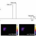
The details of the steps followed in preparing the tissue sample and acquiring the corresponding MALDI-MSI data for this study is given in another publication [11] coauthored by the author. Following are the steps involved in correlating the MRI image data of the tissue with that of the MALDI-MSI data (Figs. 8 and 9).

The original MRI image data was up-sampled (see Notes 1 and 2 ).
The HCS process was applied within the region of interest (ROI) enclosing the tissue.
The typical segmentation output was identified.
The HCS segmentation output was correlated (visually) with the MALDI-MSI (Fig. 9).

Fig. 8

Processing of the T2-weighted MRI image section (a) of the tissue specimen. The original image data is Up-Sampled (b). The HCS process relevant output highlighting the inner details of the abnormality (c, d)

Fig. 9

Correlation of the HCS process’ highlighted inner details of the abnormality with the MALDI-MS image

The primary requirement of an automated abnormalities detection system (like HCS) is the segmentation of the potential abnormal regions from noise and background. Segmentation of regions of abnormalities in images of low resolution is a challenging task. However, still, from the output in Figs. 8 and 9 one can infer that there is a potential for this approach (see Note 6 ).

3.3 HCS Process as a Perception Aid in Delineating Abnormalities in X-Ray Mammograms

Computer-aided detection (CAD) systems offer prompts to alert the reader to potential abnormalities. Hierarchical Clustering-based Segmentation (HCS) goes further by identifying the more appropriate edges of a lesion and heterogeneous regions within. The following method was adopted to evaluate how the HCS process outputs aid in the visualization of the details within the abnormalities in X-ray mammograms.

Since the main aim is to aid the user to visualize the finer details of an abnormal region, to start with the approximate location and extent of the abnormality is marked by the user (Fig. 10).

Fig. 10

Part of the original X-ray mammogram image with the part of the image having the abnormality enlarged
Since the original image data is of very high resolution and since the HCS process is processing intensive the original image data was subsampled (see Notes 3 and 4 ) (Fig. 11).

Fig. 11

Original size of the part of the image containing the abnormality and a reduced size of it after applying bilinear subsampling to the original data
The HCS process was applied to the subsampled image data within the ROI and for the HCS process’s relevant segmentations following three types of output were created (see Note 7 ).

Boundary outlined dissimilar regions (Fig. 12).

Fig. 12

HCS process’ boundaries outlining the, hard to visualize, finer inner details of the abnormality

Heat map of the dissimilar regions (Fig. 13).

Fig. 13

Heat map image of the different dissimilar regions, within the abnormality, found by the HCS process

Highlighted dissimilar regions (Fig. 14).

Fig. 14

Highlighted parts of the abnormality which are found to be dissimilar from the surrounding region

We set out to determine whether the HCS process’s output would be useful and offer a potential computer-based decision aid in that it can aid in the identifying of the appropriate edges of a lesion and heterogeneous regions within that lesion area.

An initial pilot study was conducted as an online study.

[https://shusls.qualtrics.com/SE/?SID=SV_20oJptApsrst2xT].

The study participants were asked a few standard demographic questions and a couple of questions regarding their current use of computer-aided detection when interpreting mammograms . In the main task of the study the participants were presented with six mammograms, with a region of interest containing a suspected lesion already marked [12].

In condition 1, they were asked to examine this region and to indicate the extent of the lesion by using the mouse to place markers on the outer edges of the lesions. Participants were then asked whether or not they thought the lesion was multifocal and whether they thought it might be malignant.

In addition to the images shown on the screen, the original DICOM images were made available for them to download if they wish. After completing this they were then asked to repeat the task, but this time taking into consideration the additional information provided by the HCS process’s output aids (condition 2) [12].

In the pilot study, the absolute differences in lesion measurements and the inter-subject reliability were compared between the two conditions. The intraclass correlation coefficient was used as an estimate of reliability and was similar between the two conditions (0.59, 0.57) [12].

Only gold members can continue reading. Log In or Register to continue