Fig. 20.1
The term “crossing fibers” can refer to any situation where the fiber orientation is not unique. This includes obvious cases where the voxel contains two fiber bundles that cross or pass close to each other (left), but also voxels where the fibers themselves are curved, such as curving or diverging configurations (right), or any combination of these two (middle)
Fig. 20.2
A simple illustration of the effect of crossing fibers in diffusion tensor imaging. The diffusion tensor model is a good fit for voxels that contain a single fiber orientation (left and middle columns), but fails to capture the orientation information when two distinct orientations are present (right); in this case, the major eigenvector will not in general be aligned with either of the populations present, and the anisotropy is also reduced. On the other hand, the DW signal itself (bottom row) clearly does contain higher-order information in crossing fiber voxels (bottom right), which can be used to resolve the different fiber orientations present
The fact that the diffusion tensor is affected by the crossing fiber problem has been known since its very invention [12]; however, it is only recently that the scale of this problem has been fully appreciated. Recent work demonstrates that multiple fiber populations can be detected in over 90 % of imaging voxels in the white matter [13]. The scale of this problem has obvious and profound implications for both DTI-based tractography techniques and DTI-derived measures used to assess tissue integrity.
The impact of crossing fibers has important ramifications for the application of tractography in particular, as the DTI model provides incorrect fiber orientation estimates in regions containing complex fiber configurations (see Fig. 20.2) [1]. This has important practical implications, as the majority of white matter tracts will traverse regions with multiple fiber orientations at some point along their path. Even a single incorrect orientation estimate (or for that matter, even a relatively small error in orientation estimation) will be enough to cause the algorithm to veer off-course or follow a completely unrelated tract, resulting in the delineation of false negative [13, 14] or false positive delineation of white matter pathways [13, 15]. The severe limitations of using the diffusion tensor model for fiber tractography have consistently been reported in the neurosurgical literature [16–20]. Of particular concern is that studies that have specifically investigated the feasibility of DTI-based tractography for the purpose of visualizing tracts of neurosurgical interest demonstrate that these methods result in systematically unreliable and clinically misleading tractography information [17, 19].
The extent of the crossing fiber problem means that caution also needs to be observed when interpreting DTI-derived diffusion indices such as fractional anisotropy (FA ), particularly if the intention is to use them as surrogate markers of white matter “integrity” [11, 21–23]. It is well known that FA values vary greatly over the white matter even in healthy controls where there is no known change in white matter integrity. Such variations are likely due to the presence of crossing fibers in different parts of the white matter leading to reductions in tensor-derived anisotropy, as was originally suggested in the early DTI literature [24]. The profound confounding influence of crossing fibers on the interpretation of DTI-derived diffusion indices in the presence of pathology is demonstrated in clinical studies that have observed an increase in anisotropy in cases where the given pathology or condition would have been expected to result in a reduction in tissue integrity [25]. The diffusion tensor model is increasingly recognized to be a gross over-simplification of the actual anatomy and the simplistic interpretation of DTI derived indices as a marker of white matter “integrity” is fraught with technical challenges [22, 23, 26]. As a consequence, there is a growing interest in finding clinically feasible alternatives to DTI [27].
Over the past decade, more advanced models have been developed to specifically address the limitations of the DTI model ([5–7], see reviews in [8]), many of which are now being used clinically with promising results. In this section, we describe some of the concepts and theory behind approaches that are based on high angular resolution diffusion-weighted imaging (HARDI) data [4], developed specifically to provide more robust fiber orientation estimates for applications such as diffusion tractography, and more recently to provide more biologically accurate measures of tissue microstructure or “integrity.”
HARDI Methods
What Is HARDI?
The term HARDI stands for high angular resolution diffusion imaging, and was originally coined by Tuch et al. to refer to the particular acquisition strategy employed in their study, namely the use of dense sampling on the sphere using a single b-value , as illustrated in Fig. 20.3 [4]. Data acquired in such a way allow the thorough characterization of the angular dependence on the DW signal, with no attempt at characterizing its radial (b-value) dependence. For this reason, it is arguably the most efficient acquisition strategy for the purpose of fiber orientation estimation, and hence for tractography.
Fig. 20.3
The motivation for HARDI is the need to capture all the features of the DW signal over the sphere. For example, the DW signal shown on the right clearly contains angular features, and these features are key to resolving crossing fibers. The idea behind HARDI is to sample the orientation space as densely and uniformly as is practical, using a suitable set of DW directions such as those shown on the left. By measuring the DW signal along these orientations (middle), the DW signal can be reconstructed by fitting a surface (right), so that these features can be estimated accurately
The HARDI acquisition is essentially identical in nature to the standard DTI acquisition, and differs only in that a larger number of unique diffusion-weighting gradient directions are used, potentially using a larger b-value than would be considered optimal for DTI. There is in fact no clear point at which an acquisition strategy becomes a HARDI sequence or vice-versa. For example, the current recommended minimum number of directions for robust DTI is 30 [28], while higher-order reconstruction methods have been applied to data acquired using as few as 20 directions [29]. Nonetheless, a sequence will typically be considered HARDI if the number of directions is relatively large (>~40).
It is worth noting that HARDI is not in itself a method for estimating fiber orientations; it refers specifically to the acquisition strategy. This can lead to confusion in the literature when authors claim to “perform a HARDI reconstruction”—this statement is ambiguous since it makes no mention of the reconstruction method used: it is in fact perfectly possible to perform a DTI reconstruction using HARDI data. Nonetheless, HARDI is the most common data acquisition strategy required for methods that aim to resolve crossing fibers, and for this reason the term HARDI is often used to refer to more advanced higher-order methods.
Why HARDI?
The simplest and most intuitive approach to understanding HARDI is to consider the example shown in Fig. 20.2, with two fiber populations crossing within a voxel. In this example, it is easy to see that DTI provides a good characterization of each of the two fiber populations separately, but fails when the two are combined. However, if we focus on the DW signal itself, it is clear that there is structure present in this case that the tensor ellipsoid fails to capture. Indeed, the DW signal for the crossing fiber case is to a very good approximation the sum of the DW signals that would be measured for each population independently; even by eye, the two contributions can easily be appreciated in the combined DW signal. The aim of HARDI methods is essentially to separate out these two contributions, and thus to resolve crossing fibers. For this to be possible, the relevant features of the DW signal need to be captured with sufficient accuracy. This requires a larger number of DW directions than typically acquired in DTI, leading directly to the development of HARDI approaches.
The problem of separating the two contributions can in essence be written out as a set of simultaneous equations: M DW measurements are acquired per voxel, and from these a set of N model parameters need to be estimated. What these N parameters represent is dependent on the particular reconstruction approach used: they might represent the orientations and volume fractions of a fixed number of potential fiber populations, or the coefficients of a more continuous representation of the diffusion or fiber configuration, as illustrated in Fig. 20.4. The latter is particularly advantageous from a mathematical perspective, since describing the orientation information using a continuous distribution allows the problem to be expressed and solved using extremely fast linear algebra techniques, with reconstruction times on the order of seconds for whole-brain datasets. Using a more explicit parametric representation (for example partial volume and orientation per fiber population) does not lend itself to such convenient linear approaches, and will in general necessitate the use of more computationally expensive nonlinear optimization methods.
Fig. 20.4
The simplest approach to modelling crossing fibers in HARDI is to assume that the DW signals from the various fiber populations add up to give the total measured DW signal for that voxel (middle left). Resolving these crossing fibers is then a matter of finding the fiber configuration that best matches the observed data. One way to represent this configuration is as a set of discrete orientations with associated volume fractions (left); this is approach used in multi-tensor fitting methods. Another approach is to represent the fiber configuration as a continuous distribution, which can be approximated by a dense set of fixed orientations and corresponding volume fractions (right); this is the approach used in spherical deconvolution methods
Using HARDI to Resolve Crossing Fibers
By far the most common application for HARDI methods is the estimation of the fiber orientations for use in fiber tracking. A number of methods are available to achieve this, but all are based on the same concept: each fiber population (i.e., distinct orientation) adds its own contribution to the measured signal, so that the total measured signal is the sum of the contributions that would have been measured for each bundle in isolation.
Multi-Tensor Fitting
Based on this observation, the most obvious approach to resolving crossing fibers is the multi-tensor approach: we assume the voxel contains two fiber populations rather than one, with each population modeled using its own diffusion tensor. In this case, the minimum additional information required is the relative amounts of each fiber population (i.e., their volume fractions) and their respective orientations. The problem is then one of estimating the set of parameters (volume fractions and orientations) that best fit the measured data [4, 30].
It turns out that this is not a simple problem to solve in practice due to the nonlinear formulation of the problem (a sum of exponentials), dictating the use of computationally expensive nonlinear minimization methods . In addition, the problem is generally ill-conditioned, due to the difficulty of differentiating between changes in anisotropy and changes in volume fraction of the constituent fiber populations1; to get around this, most implementations enforce the condition that each diffusion tensor be at least axially symmetric, and often hold all their diffusivities constant (i.e., assume a fixed mean diffusivity and anisotropy). Nonetheless, a number of methods are based on this general approach; some allow for larger numbers of fiber populations, some include an isotropic “CSF” compartment, and some use advanced Bayesian Monte Carlo Markhov Chain (MCMC) sampling techniques to characterize the uncertainty about the parameters estimates [14, 30–32].
The Combined Hindered and Restricted Model of Diffusion (CHARMED) approach is strongly related to the multi-tensor approach in that it also models each fiber population independently [33, 34]. However, it differs substantially in that it assumes a more biologically plausible model of restricted diffusion in cylinders to represent the DW signal from each fiber populations, rather than a diffusion tensor model. It also includes an extracellular compartment, itself modeled by a diffusion tensor. One limitation is that it requires a more demanding multi-shell (i.e., multiple b-values) HARDI data acquisition, leading to lengthier scan times.
One issue with these methods is that they somehow need to know how many fiber populations to include in the model for each voxel. While a number of approaches have been proposed to do this [2, 14, 31], any errors in this number will inevitably lead to errors in the estimated parameters. Most of these approaches are based on some statistical “goodness of fit” measure, and this will in general lead to underestimation of the number of fiber populations present, particularly in noisy data where any improvements in the model fit will be overwhelmed by the noise. The result is that while the algorithm can be said to be “conservative” in that it only includes additional fiber populations if there is good evidence that these are needed, it will inevitably fail to identify a significant proportion of crossing fiber voxels and therefore model them using the single tensor model , with all the limitations highlighted above.
Spherical Deconvolution
The multi-tensor approach can be extended by switching from a discrete representation (i.e., a small number of distinct fiber populations) to a continuous representation of the fiber orientation information. One way to understand this is to imagine that rather than trying to estimate the volume fraction and orientation of each fiber population, we are now going to model a large number of fiber populations, each with a fixed orientation. The problem now reduces to figuring out the volume fractions of each of these. If we use a sufficiently dense set of orientations that are uniformly distributed over the sphere, the information can be represented as a distribution of volume fractions over the sphere, as illustrated in Fig. 20.4. This distribution is commonly referred to as the fiber orientation density function (fODF ) or simply the fiber orientation distribution (FOD ).
Essentially, the FOD is a function defined over the sphere, which represents the amount of fibers at any point on the sphere (i.e., aligned with the corresponding orientation). It is often displayed using orientation plots such as those shown in Fig. 20.5, whereby the distance from the origin represents the “density” along the corresponding orientation. Distinct fiber orientations can clearly be seen as distinct peaks in the FOD.
Fig. 20.5
Fiber orientation distributions obtained from a healthy volunteer, estimated using constrained spherical deconvolution [29] as implemented in MRtrix [35]. These are shown as a coronal projection overlaid on the mean DWI image, with the corpus callosum clearly visible in the centre with fibers running left–right (red lobes). Its lateral projections can be seen to cross through the fibers of the corona radiata (running inferior–superior; blue lobes) and the superior longitudinal fasciculus (running anterior–posterior; green lobes)
The advantages of using such a distribution to represent the fiber orientation information are threefold. First, it means that the relationship between the measured DW signal and the FOD is linear, allowing the use of much more efficient reconstruction methods based on linear algebra . Second, there is no need to specify the number of directions that might be present in each voxel; the FOD is continuous, and distinct fiber orientations will simply be reflected as distinct peaks in the FOD. Finally, the FOD is suited to describing fiber configurations containing a range of orientations, such as for example bending or fanning fibers; these are clearly not well characterized using a single orientation, as would be used in multi-tensor approaches. In these cases, the corresponding peak in the FOD will simply be broadened accordingly, as expected. Spherical deconvolution approaches are therefore more computationally efficient, while providing a much more general description of the fiber orientation information. These provide estimates of the FOD that are suitable for fiber-tracking , as illustrated for example in Fig. 20.6.
Fig. 20.6
Whole-brain fiber- tracking results obtained from a healthy volunteer, generated using a probabilistic fiber tracking algorithm on orientations estimated using constrained spherical deconvolution [29] as implemented in MRtrix [35]. A 2 mm-thick section through the tracks is shown as a sagittal projection. Amongst other white matter tracts, the superior longitudinal fasciculus can be seen running anterior–posterior (green) and then down into temporal and parietal regions. Also visible are the uncinate fasciculus, connecting the temporal pole to the frontal lobes (blue), and the inferior fronto-occipital fasciculus running anterior–posterior (green), connecting the frontal lobe to the occipital lobe
A number of different spherical deconvolution techniques have been proposed [10, 29, 36–39]. The most stable of these impose a non-negativity constraint to explicitly prevent or minimize negative fiber density values, which are clearly non-physical; this has been shown to dramatically improve the robustness to noise of these methods [29, 37]. Some estimate the per-fiber anisotropy on a per-voxel basis [36], other assume fixed diffusivity values [37–39], while others bypass the diffusion tensor model entirely and measure the actual per-fiber DW signal profile from the data themselves [10, 29].
The “Constant Anisotropy” Assumption
The overwhelming majority of multi-tensor fitting and spherical deconvolution techniques will make the assumption that all fiber bundles can be described by diffusion tensors with the same intrinsic “constant anisotropy” (or at least axial symmetry) to reduce the complexity of the problem. At first sight, this might seem to be a gross over-simplification, particular to those steeped in the more traditional DTI framework, where tensor-derived metrics are often used as surrogate markers of white matter “integrity.” Since these new approaches assume fixed values for these metrics over all white matter bundles, it is now impossible to estimate equivalent measures, let alone detect differences between them.
However, there are very good reasons to believe that this approximation holds in most, if not all cases. The assumption of fixed anisotropy inherently implies that all observed anisotropy differences in the brain are due entirely to crossing fiber effects or other partial volume effects (e.g., with CSF). This is in fact in line with the original DTI literature, where the large variations of anisotropy observed in healthy volunteers were attributed to differences in the coherence of fiber tract directions [24]. The relationship between anisotropy (and more recently radial and axial diffusivities) and white matter “integrity” was suggested based on highly controlled single nerve experiments, where any confounding effects of crossing fibers could explicitly be ruled out [40–44]. While these studies undeniably demonstrated changes in various tensor-derived metrics under different conditions (dysmyelination, axonal injury, changes in axonal diameter, etc.), these changes are dwarfed by the changes induced by the presence of crossing fibers [1, 23]. Moreover, and more importantly, while changes in diffusivities and/or anisotropy can be observed in these experiments, they are not of a magnitude sufficient to alter the results dramatically; as shown in previous studies, while moderate changes in the assumed anisotropy will affect the estimated volume fractions, they have almost no impact on the estimated fiber orientations [10]. In fact, any pathology that would cause severe changes in the anisotropy of the per-fiber DW signal would probably need to involve destruction of the axonal membrane, with a large increase in radial diffusivity and corresponding reduction in the DW signal; this will be interpreted by these models primarily as a dramatic decrease in volume fraction, an interpretation that is in fact fairly accurate given the pathology.
For this reason, this particular assumption is very commonly employed, and with great success. However, the implication is that genuine anisotropy changes are at best extremely difficult to detect from HARDI data (given that they are essentially indistinguishable from partial volume effects), which essentially rules out the possibility of deriving equivalent markers of white matter “integrity”—at least using these approaches. Instead, the current trend is to focus on the estimated partial volume fractions, since these seem to have the most dominant impact on the DW signal, and can be used as estimates of fiber density—a measure that, although different from the more common interpretation of “integrity,” is nonetheless clearly clinically very relevant [45–47].
Using HARDI to Characterize Diffusion
Another approach to the crossing fiber problem is to take a step back and focus on characterizing the diffusion process itself, rather than the fiber configuration directly. The motivation for such approaches is to avoid over-interpretation of the measured data. The relationship between the measured DW signal and the actual fiber configuration and associated tissue composition is obviously extremely complex: white matter is not made up of neatly arranged impermeable cylinders, but contains a wide range of different cells of different sizes and shapes, each with their own internal microstructure. Clearly, the DW signal depends on a myriad of different factors, and any attempt at extracting specific microstructural information will inevitably require that assumptions and approximations be made. Rather than trying to do this, it might be best to characterize what we can, and avoid making any potentially invalid or unjustified assumptions. For this reason, a number of so-called model–free techniques have been proposed to characterize the diffusion process itself.
q-Space and the Spin Propagator
These methods are all in some way based on the theory of q-space [48], which describes the relationship between the DW signal and the so-called average spin propagator (also called the spin displacement probability density function ). In simple terms, the spin propagator is a function describing the probability P(r|x,Δ) that a water molecule initially at x has moved by displacement r during the diffusion time Δ of the MR measurement. For free diffusion, this is simply a Gaussian distribution with standard deviation equal to the root mean square displacement of the water molecules (as per Chap. 3). For more complex environments, the propagator will have a more complex shape, as illustrated in Fig. 20.7. This makes no assumption about whether diffusion is free or restricted: it simply characterizes the chances of molecules moving along a given direction by a given amount. In general, this will depend on the diffusion time Δ: with free diffusion, the distances moved will increase with diffusion time. However, in restricted geometries the maximum distance moved will clearly be dictated by the size of the restricting compartment. The relationship between the DW signal and the spin propagator is relatively simple and not subject to any particular biological assumptions.2 Clearly, the diffusion propagator provides the most complete and accurate description of the diffusion process, and contains all the information that can be extracted from diffusion MRI, which is the reason why a number of methods attempt to estimate it.
Fig. 20.7
Illustration of the relationship between the fiber configuration (left), the average spin propagator (middle), and the diffusion ODF (right). In a crossing fiber voxel (left), water molecules will tend to diffuse more readily along the fiber orientations than across them. This corresponds to a spin propagator with pronounced “ridges” along the fiber orientations (middle). This is a full three-dimensional density function, the characterization of which requires a vast amount of data. In contrast, the diffusion ODF (right) provides a more condensed version of spin propagator, which essentially describes the probability of a water molecules moving along any given orientation. As expected, the peaks of the dODF point along the fiber orientations
According to q-space, the DW signal is related to the spin propagator via a simple Fourier transform. In practice, this means that to estimate the spin propagator along one dimension, a number of DW images need to be acquired, each with a different q-value.3 To get an accurate estimate, a sufficient number of distinct q-values need to be acquired, up to a sufficiently large maximum q-value to ensure near-complete nulling of the DW signal. These two requirements alone are difficult to achieve: for a full three-dimensional characterization of the spin propagator, the number of distinct q-vectors (and hence image volumes) required is of the order of 1000 (approx. 10 per image axis). These requirements also dictate the use of very large gradients and/or long echo times (to achieve the very large maximum q-values needed), leading to a reduction in the SNR. Clearly, the full characterization of the spin propagator is extremely challenging.
Nonetheless, this complete characterization is exactly what Diffusion Spectrum Imaging ( DSI ) aims to achieve [49]. To do this, 515 image volumes are acquired, each with a distinct q-vector with a maximum b-value of 17,000 s/mm2. This is clearly a much more demanding acquisition than can realistically be accommodated in routine clinical imaging, and for this reason much of the recent development in this area has been focused on obtaining relevant features of the spin propagator (namely the diffusion orientation density function; dODF) using the much more clinically achievable HARDI acquisition.
The Diffusion Orientation Density Function (dODF )
Essentially, the dODF is a simplified version of the full spin propagator, which provides only the probability of a water molecule moving along a given direction; any information about how far it moved is discarded. This much more compact version of the spin propagator is obviously still sufficiently informative, especially for the purposes of resolving crossing fibers, motivating the development of these HARDI-based methods.
Q–ball Imaging (QBI ) was the first method proposed to estimate the dODF [50]. It performs a Funk–Radon Transform on the HARDI data to map the DW signal per-voxel onto the corresponding dODF. This has the advantage of being a linear operation, and was subsequently shown to be much more efficiently and robustly implemented using spherical harmonics [51, 52]. More recently, Constant Solid Angle Q–ball Imaging (CSA -QBI ) has been proposed to obtain a more accurate , sharper estimate of the dODF [53].
Other techniques based on q-space that have been proposed include the Diffusion Orientation Transform (DOT ), which provides a contour of the spin propagator evaluated at a particular value of the displacement—in other words, it provides the probability of a water molecule moving along any given direction by a fixed distance [54]. Another early technique is Persistent Angular Structure MRI (PAS-MRI ), which evaluates an ODF from relatively modest data by imposing a maximum entropy constraint [55]. See Fig. 20.8 for an illustration of the results obtained using three different dODF estimation methods.
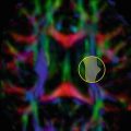
Fig. 20.8
An illustration of the results obtained using three different dODF estimation methods: Q-ball imaging (QBI; left), constant solid angle QBI (CSA-QBI; middle), and the diffusion orientation transform (DOT; right). These are displayed as coronal projections overlaid on the fractional anisotropy map, showing the well-known crossing of the lateral projections of the corpus callosum (left–right) with the corona radiata (inferior–superior) and the superior longitudinal fasciculus (anterior–posterior) [Reprinted from Aganj I, Lenglet C, Sapiro G, Yacoub E, Ugurbil K, Harel N. Reconstruction of the orientation distribution function in single- and multiple-shell q-ball imaging within constant solid angle. Magn Reson Med. 2010 Aug;64(2):554–66. With permission from John Wiley & Sons.]
The Narrow Pulse Approximation
The theory of q-space does rely on one approximation: that the duration of the DW gradient pulses is negligible—in other words, the DW gradient pulses can be considered to be infinitesimally narrow. More specifically, the distance moved by molecules during the application of each DW gradient pulse should be much smaller than the distance moved between the pulses. The idea is that each DW gradient pulse respectively “tags” and “untags” water molecules based on their current location, so that the only relevant quantity is their actual displacement between these two events. For this approximation to hold in white matter, water molecules should not be allowed to diffuse by any distance approaching the axonal diameter. Even if we assume an acceptable distance to be 1 μm (which is already larger than many axons) and a diffusion coefficient of 10−3 mm2/s (which is smaller than would typically be assumed), the DW pulse duration would need to be less than 0.5 ms. To achieve any reasonable b-value with such a short pulse duration would require gradients strengths and rise-times orders of magnitude larger than can be used in the clinic. In practice, the minimum DW pulse duration than can realistically be achieved on a human system is of the order of 10 ms. Clearly, the narrow pulse approximation cannot hold on a clinical system.
Related posts:

Stay updated, free articles. Join our Telegram channel

Full access? Get Clinical Tree


