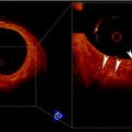
Hypothesis Validation of Far Wall Brightness in Carotid Artery Ultrasound for Feature-Based IMT Measurement Using a Combination of Level Set Segmentation and Registration

Fig. 21.1

(a) Original B-mode image. (b) Downsampled and despeckled image. (c) Convolution of image (b) with a first-order Gaussian kernel. (d) Automated tracing of the far adventitia layer (AD_F) in image (a)

Convolution with higher order derivative: We filtered the image (Fig. 21.1bb) by using a first-order derivative Gaussian filter (Fig. 21.1cc). This filter is the equivalent of a high-pass filter, which enhances the representation of the objects having the same size of the kernel. Since we aimed at enhancing the representation of the carotid walls, we chose a kernel size of 8 pixels.

Heuristic search for AD_F: Starting from the bottom of the image, the far carotid wall was recognized as it was a bright stripe of about 8 pixels size (Fig. 21.1dd). As mentioned in step 1, the nominal value of the IMT is about 1 mm which is equivalent to 8 pixels in the downsampled domain. Thus, the first-order Gaussian derivative kernel is size matched to the IMT and it outputs a white stripe of the same size as the far wall thickness. Our heuristic search considered the image column-wise. The intensity profile of each column was scanned from bottom to top (i.e., from the deepest pixel moving upwards). The deepest region which had a width of at least 8 pixels was considered as the far wall.

Guidance zone creation: The output of this carotid recognition stage was the tracing of the far adventitia layer (AD_F) (a complete description of this procedure is given in [13]). We selected a Guidance Zone (GZ) in which we performed segmentation. The basic idea was to draw a GZ that comprised the far wall (i.e., the intima, media, and adventitia layers) and the near wall. The average diameter of the carotid lumen is 6 mm, which roughly corresponded to 96 pixels at a pixel density of 16 pixels/mm. Therefore, we traced a GZ that had the same horizontal support of the AD_F profile, and a vertical height of about 200 pixels. With this vertical size, which is double the normal size of the carotid, we ensured the presence of both artery walls in the GZ.

Lumen segmentation: The lumen segmentation consists of a preprocessing step followed by a level set based segmentation method. The first preprocessing step is the inversion of the image, i.e., we subtract every pixel in the image from the maximum value of the image. We then multiply the image by a function of the gradient of the original image given by (21.1) below.

$f(\nabla u)=\frac{1}{{1+\left| {\nabla u} \right|}}$

(21.1)

Here u indicates the image. The function is such that it takes low values (≪1) at the edges in the image and takes a maximum value of 1 in regions that are “flat.” The lumen is then segmented using the active contour without edges algorithm or the Chan–Vese algorithm as described in [14] (Appendix). The algorithm was chosen because of the piecewise constant nature of the cropped carotid artery images obtained from the previous step. The lumen, after preprocessing, is white and its grayscale intensity is high (>100) with noise. The walls of the artery that initially appear bright become dark (i.e., <50 grayscale intensity) after preprocessing. The Chan–Vese method is very effective for segmenting images made up of two piecewise constant regions which in our case correspond to the lumen and the carotid wall. The segmentation produces a binary image where the lumen is white (intensity of 1) and the wall intensity is 0. We would also like to point out that the algorithm is not influenced by the actual gray scale values in the carotid images giving us the flexibility to analyze images acquired with different settings. The algorithm is also robust to noise as it does not directly depend on the edges in the images. The pseudo-code for the entire automated segmentation algorithm is as follows:

(A)

Invert image, i.e., subtract image from maximum value in the image.

(B)

Multiply with function given in (21.1).

(C)

Downsample image by a factor of 4. Since numerical Partial Differential Equations require long computing times, we downsampled the image to achieve convergence in a reasonable amount of time.

(D)

Initialize level set contour as a rectangle. The initial contour placement is automated. We computed a rectangular contour centered on the image.

(E)

Run the Chan–Vese algorithm for 1,000 iterations. The number of iterations was arrived at by trial and error and it was sufficient for all test images across different databases.

(F)

Upsample the segmentation result, which is a binary image where the lumen is 1, to the original size of the image.

(G)

The presence of the jugular vein in some images causes the algorithm to segment both the carotid and the vein. In this case, employ a connected component analysis to determine which connected group is closer to the AD_F. The connected group closest to the AD_F is taken as the carotid artery.

(H)

Apply morphological hole filling to remove holes in the binary segmentation result caused by the backscatter noise in the lumen.

3.2 Image Alignment for Composite Image Generation

The first step in the automated IMT measurement algorithms like CALEX is the recognition of the Common Carotid Artery (CCA). For this purpose, the assumption by most of these feature-based algorithms is that the far wall of the CCA has the highest intensity in the image. To validate this assumption, it is necessary to locate the far wall and determine its intensity. If the ultrasound probe is exactly along the longitudinal axis of the CCA, the resulting image will show a nearly horizontal straight CCA with respect to the base edge of the image. However, not all CCA images are acquired parallel to the longitudinal axis. Sometimes, the probe can make a slight angle with the longitudinal axis of the CCA, and therefore, the resultant image will not have the CCA absolutely horizontal with respect to the base of the image. Such images will show a slightly tilted CCA. In order to superimpose all these images to show that the cumulative far wall intensity is the highest, we register all CCA images with respect to an ideal image in which the CCA is parallel to the base edge. This is the main motivation for registering the images in our work.

A near straight artery image is used as a target image for all other images in the database. Lumen segmentations of binary images are affine transformed to estimate the rotation and translation of the floating image into the same orientation and position as target image. The free form deformation registration method using B-spline described in [15] was used for nonrigid registration. The method is a hierarchical transformation model where the local deformations are described by free form deformations modeled using B-splines. Registration is performed by minimizing a cost function that is a combination of sum of squared differences and a cost function associated with the smoothness of the transformation. The free form deformation based on B-splines deforms the object by altering an underlying mesh of spline control points. The alteration produces smooth and continuous transformations. In two dimensions, we denote x and y as the coordinates of the image volume. Let φ _ijdenote the mesh of control points (n ₁ × n ₂). The deformations produced by the B-splines can be written as

$\begin{aligned} d(x,y,z)&=\sum\limits_{l=0}^3 {\sum\limits_{m=0}^3 {{B_i}(u){B_j}(v)\varphi{_{i+l,j+m }}} } \hfill \\ i&=\left\lfloor {\frac{x}{{{n_1}}}} \right\rfloor -1,\kern0.75em j=\left\lfloor {\frac{y}{{{n_2}}}} \right\rfloor -1 \hfill \end{aligned}$

(21.2)

In (21.2), B _l represents the basis functions of the B-splines, given by (21.3):

$\begin{aligned} {B_0}(u)&=\frac{{{(1-u)^3}}}{6} \hfill \\ {B_1}(u)&=\frac{{(3{u^3}-6{u^2}+4)}}{6} \hfill \\ {B_2}(u)&=\frac{{(-3{u^3}+3{u^2}+3u+1)}}{6} \hfill \\ {B_3}(u)&=\frac{{{u^3}}}{6} \hfill \end{aligned}$

(21.3)

The cost function for the registration is mathematically given as

$\begin{array}{lll} C&={{\sum {(I-T(F))}}^2}\\ &\quad +\sum\limits_x {\sum\limits_y {\left[ \begin{array}{lll} {{\left( {\frac{{{\partial^2}d}}{{\partial {x^2}}}} \right)}^2}+{{\left( {\frac{{{\partial^2}d}}{{\partial {y^2}}}} \right)}^2}+2\left( {\frac{{{\partial^2}d}}{{\partial x\partial y}}} \right) \end{array} \right]} }\end{array}$

(21.4)

where I is the fixed target reference image, and F is the floating image transformed by T (combined rigid and nonrigid transformation). The deformation d is defined in (21.2) and the derivatives are with respect to spatial coordinates. In (21.4), the second term is the penalty term for smooth deformations and is the bending energy of a thin plate of metal. The optimization solves for the control point grid from which the deformations are calculated.

Nonrigid registration using B-splines based free form deformations is one of the popular methods for nonrigid registration of multi-modality images. The algorithm’s main advantage compared to other methods is that it produces very smooth deformations due to B-splines and the transformed images are not overly distorted. Because of its use in multi-modality registration, information theoretic metrics are used as the cost function. For our application, we used the least squares criterion as we were registering 2D binary images oriented differently. It proved to be more effective than directly registering the grayscale carotid artery images. Several implementations of this algorithm are readily available in various languages. We used the Matlab implementation by Dr. Dirk-Jan Kroon available from Mathworks file exchange. The algorithm is generally slow (5 min per image pair). But in our case we are using it only for validation purposes and will not be a part of any commercial implementation. We also perform an initial affine registration that scales and aligns the floating image. The nonrigid registration is the final step to obtain a more accurate transformation field.

4 Segmentation and Registration Performance

4.1 Segmentation and Registration Results

The average distance between the manually traced Media–Adventitia (MA) boundary and the automatically traced AD_F was 25.03 ± 19.47 pixels (1.54 ± 1.19 mm). This small distance indicates that the automatically traced AD_F profile and the manually traced MA profile match, and therefore, the recognition of the carotid artery was successful. The segmented lumen of the fixed base carotid artery and a floating carotid artery image belonging to different patients are shown Fig. 21.2. The images are chosen to highlight the requirement for an affine transformation prior to a nonrigid registration.

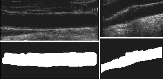
Fig. 21.2

Segmentation results. Fixed reference image of carotid artery (top left) and one of the 200 floating carotid artery images (top right). Binary image of segmented fixed reference image lumen (bottom left) and binary image of segmented floating image lumen (bottom right)

In Fig. 21.3, a typical registration result is shown. We have chosen two carotid artery images that were at an angle with respect to the horizontal. The transformation is the result of an affine transformation followed by the free form deformation. We chose a weighting factor of 0.01 for the smoothing term in the cost function. Typically, it took about 35 iterations for the affine registration to converge. Following affine, the nonrigid registration took 60 iterations to converge.

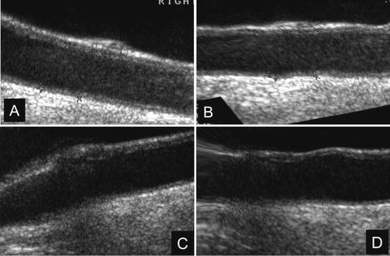
Fig. 21.3

Result of nonrigid free form deformation of two carotid artery images with the carotid artery at an angle with respect to the horizontal. (a) and (b) are the acquired and transformed image pairs of one carotid artery. Similarly (c) and (d) are acquired and transformed image pairs of the second carotid artery

In Fig. 21.4, a surface plot of the sum of all registered images is shown. The grayscale sum image is also displayed. The window and level of the grayscale image are set to its minimum and maximum values. The results in Fig. 21.4 confirm our hypothesis qualitatively. To obtain quantitative evidence, we calculated the maximum value along every column in the sum image and confirmed that the maximum value along each column was from the far wall. In Fig. 21.5, the mean intensity and standard deviation from a 5 × 5 window centered on the same column along the near and far wall are shown. The far wall intensity is clearly higher and well separated from the average values along the near wall. A z-score was calculated by dividing the difference between the mean values of the corresponding 11 × 11 window along the far and near walls and sum of their standard deviations. For all windows considered, the z-score was greater than 2.

Fig. 21.4

Surface plot of the registered sum of 200 images showing intense far wall (left). The same displayed as a 2D image (right). The top row image is the result of nonrigid registration while the bottom row image is the results using affine registration. The arrows point to the far wall

Fig. 21.5

Mean intensity and standard deviation along the far wall and near wall

4.2 Far Wall Brightness Hypothesis Validation and Discussion

In this work, we validated the hypothesis of far wall maximum brightness using a much larger dataset comprising of 200 images. Our approach was to register all the B-mode US images to a base fixed image which is considered carotid “straight.” The US images of the carotid artery do not have many structures and there are no landmarks that can be used to assess the quality of registration. We used the intensity sum image to verify that the lumen volumes coincided. Since we used a nonrigid registration algorithm, we manually verified that the deformations are smooth and do not overly distort the carotid artery. Since the artery in different patients can be oriented at different angles and consequently be of different lengths in the image, we require an affine transformation to orient and scale the arteries appropriately. The nonrigid transformation aligns the edges of the segmented lumen. In many cases, nonrigid registration might not be required as the artery images are straight and do not have any distortions.

The registration accuracy in terms of sub-pixel metrics is not a hard requirement for this work. We wanted to verify that the far wall has higher intensity than the near wall in all images and for that purpose it is sufficient that the images be registered within the thickness of the far wall. Our hypothesis can be easily verified by visual inspection of Figs. 21.3 and 21.4 (3D plots). In Fig. 21.4, it can be seen that the far wall has a relatively higher intensity compared to that of the near wall. Quantitative results are depicted in Fig. 21.5, and the z-score of >2 also verifies our hypothesis.

The automated AD_F detection method proved very robust and had a 100% success rate. This ensured the possibility of an accurate segmentation, which is based on AD_F tracing. The major merits of this automated adventitia recognition is that the multiresolution stage is strictly linked to the pixel density of the image. This gave robustness to the method, as in the multiresolution framework, we always worked with a Gaussian kernel size equal to the expected IMT value.

Only gold members can continue reading. Log In or Register to continue