Image Correction Method from Unconstrained Images

Fig. 1

a Overview of the used image acquisition framework (A, B), light sources (C, D) and subjects location (E) for the UBIRIS v.2 database (courtesy of Proença and Alexandre [27]). b Schematic data collection setup for the off-angle iris images of the WVU database. The subjects head is positioned on a chin/head rest and he is asked to focus straight ahead on a LED. The camera is rotated $15^\circ$ and $30^\circ$ as measured by a protractor on a movable arm positioned under the eye (courtesy of Schuckers et al. [32])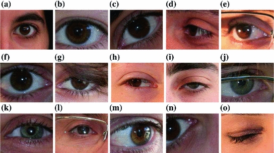

Fig. 2

Examples of UBIRIS v.2 images presenting different noise sources. See text above for a description of the “imperfections” with respect to optimal acquisitions

Images acquired at different distances from 3 to 7 m with different eye’s size in pixel (e.g. Fig. 2a, b);
Rotated images when the subject’s head is not upright (e.g. Fig. 2c;
Iris images off-axis when the iris is not frontal to the acquisition system (e.g. Fig. 2d, e);
Fuzzy and blurred images due to subject motion during acquisition, eyelashes motion or out-of-focus images (e.g. Fig. 2e, f);
Eyes clogged by hair Hair can hide portions of the iris (e.g. Fig. 2g);
Iris and sclera parts obstructed by eyelashes or eyelids (e.g. Fig. 2h, i);
Eyes images clogged and distorted by glasses or contact lenses (e.g. Fig. 2j, k and l);
Images with specular or diffuse reflections Specular reflections give rise to bright points that could be confused with sclera regions (e.g. Fig. 2l, m);
Images with closed eyes or truncated parts (e.g. Fig. 2n, o).

To verify the proposed correction method for nonideal iris recognition, we use part of the West Virginia University off-angle iris database. The dataset consists of 200 iris classes. Each class is represented by four images collected at three angles on the order of $0^\circ$ , $15^\circ$ , $30^\circ$ , and again $0^\circ$ [32]. The acquisition setup is more-constrained respect to the UBIRIS v.2 acquisition conditions: the images collected are in the near infrared range (above 700 nm) and the illumination is performed by six LEDs attached at the bottom of the camera. The schematic acquisition setup is showed in Fig. 1b and an example of four acquired images of a user are shown in Fig. 3.

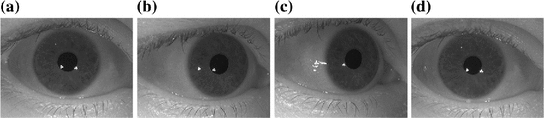
Fig. 3

Sample images from the WVU off-angle iris database. a $0^\circ$ angle; b $15^\circ$ off-angle; c $30^\circ$ off-angle; d $0^\circ$ angle

There are no eye gaze estimation algorithms working well in natural light acquisition setup [13] and moreover the WVU off-angle iris database provides a rough LoG estimation, useful to verify the proposed algorithm. On the other hand the UBIRIS v.2 database is more useful to test the sclera segmentation algorithm in non-constrained conditions.

3 Sclera Segmentation

The term sclera refers to the white part of the eye that is about 5/6 of the outer casing of the eyeball. It is an opaque and fibrous membrane that has a thickness between 0.3 and 1 mm, with both structural and protective function. Its accurate segmentation is particularly important for gaze tracking to estimate eyeball rotation with respect to head pose and camera position but it is also relevant in Iris Recognition systems: since the limbus is the boundary between the iris and the sclera, an accurate segmentation of the sclera is helpful to estimate the external edge of the iris.

3.1 Coarse Sclera Segmentation

The first step in the proposed Sclera segmentation approach is based on a dynamic enhancement of the Red, Green, Blue channel histograms. Being the sclera a white area, this will encourage the emergence of the region of interest. Calling $x_{min}$ and $x_{max}$ the lower and the upper limit of the histogram of the considered channel, assuming that the intensities range from 0 to 1, we apply, independently on each channel, a non-linear transform based on a sigmoid curve where the output intensity $$y$$

is given by:

$\begin{aligned} y=\frac{1}{1+exp\left( -\alpha \frac{x-\bar{x}}{\sigma }\right) }, \end{aligned}$

(1)

where $\bar{x}$ is the mean value of $$x$$

, $\sigma$ is the standard deviation and we assume $\alpha =10$ . The latest value is chosen making various tests trying to obtain a good contrast between sclera and non-sclera pixels.

We manually segment 100 randomly-chosen images from the whole preprocessed database, dividing pixels into Sclera ( $\omega _S$ ) and Non-Sclera ( $\omega _N$ ) classes. Each pixel can be considered as a vector in the three dimensions (Red, Green and Blue) color space $\mathfrak {R}^3$ . These vectors are then used in minimum Mahalanobis distance classifier with the two aforementioned classes, combined with Linear Discriminant Analysis (LDA) [9]. LDA projects data through a linear mapping that maximizes the between-class variance while minimizes the within-class variance [23]. Calling $\mathbf {x}$ the projected vector, corresponding to a pixel to be classified, accordingly to a minimum Mahalanobis distance criterium we define a Sclera pixel as:

$$$\begin{aligned} M_S = \left\{ {\begin{array}{*{20}c} 1 &{}{\mathtt{if }\, D_S \left( \mathbf {x} \right) \le D_N \left( \mathbf {x} \right) } \\ 0 &{}{\mathtt{if }\, D_S \left( \mathbf {x} \right) > D_N \left( \mathbf {x} \right) } \\ \end{array} } \right. \;, \end{aligned}$$” src=”/wp-content/uploads/2016/03/A320009_1_En_12_Chapter_Equ2.gif”></DIV></DIV><br /> <DIV class=EquationNumber>(2)</DIV></DIV>where <SPAN id=IEq22 class=InlineEquation><IMG alt=$ and $D_N(\mathbf {x})$ are the distances respectively from $\omega _S$ and $\omega _N$ . We recall that:

$\begin{aligned} D_i(\mathbf {x})=\sqrt{\left( \mathbf {x}-\mathbf {\mu }_i\right) ^T \Sigma _i^{-1} \left( \mathbf {x}-\mathbf {\mu }_i\right) }, \end{aligned}$

(3)

where $\mathbf {\mu }_i$ is the average vector and $\Sigma _i$ is the Covariance Matrix [9]. Therefore, using this simple linear classifier we can obtain a coarse mask for Sclera and Non-Sclera pixels using the Mahalanobis distances.

3.2 Dealing with Reflections

Specular reflections are always a noise factor in images with non-metallic reflective surfaces such as cornea or sclera. Since sclera is not a reflective metallic surface, the presence of glare spots is due to incoherent reflection of light incident on the cornea. Typically, the pixels representing reflections have a very high intensity, close to pure white. Near to their boundaries, there are sharp discontinuities due to strong variations in brightness. The presented algorithm for the reflexes identification consists mainly of two steps:

Identification of possible reflection areas by the identification of their edges through the use of a Sobel operator;
Intensity analysis within the selected regions.

The first step, using a gray-scaled version of the image, is based on an approximation of the modulus of the image gradient, $\nabla I(x,y)$ , by the Sobel $3 \times 3$ operator:

$\begin{aligned} G_x = \left[ {\begin{array}{*{20}c} { - 1} &{} 0 &{} 1 \\ { - 2} &{} 0 &{} 2 \\ { - 1} &{} 0 &{} 1 \\ \end{array} } \right] . \end{aligned}$

(4)

So $\left| \nabla I(x,y)\right| =\sqrt{G_x^2+G_y^2}$ , where $$G_y=G_x^T$$

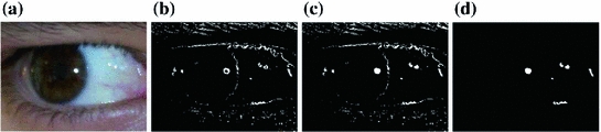
. Due to the sharp edges present on reflexes we adopt a threshold of 0.1 to define reflex edges; the threshold value is chosen as the best for the 100 images used for training. For each candidate region we then check, through a morphological filling operation for 8-connected curves [11], if it is closed, and, if this is the case, we assume it as a reflex if all pixels inside have an intensity above the 95 % of the maximum intensity present in the whole image (regions with high intensity pixels). These steps are shown in Fig. 4 where reflexes are insulated.

The location of the estimated reflections defines a “region of interest” in which the pixels are classified as Sclera or Non-Sclera following the aforementioned process. Avoiding all the pixels that are outside the “reflex regions” from the previously defined candidates for the Sclera regions provides us with the first rough estimation of Sclera Regions. Some rough results are shown in Fig. 5.

3.3 Results Refinement

A first improvement with respect to the aforementioned problems is obtained using morphological operators. They allow small noise removal, holes filling and image regions clustering. We apply the following sequence of operators:

Opening with a circular element of radius 3. It allows to separate elements weakly connected and to remove small regions.
Erosion with a circular element of radius 4. It can help to eliminate noise still present after the opening and insulate objects connected by thin links.
Removal of elements with area of less than 4 pixels.
Dilation with a circular element of radius 7 to fill holes or other imperfections and to join neighbor regions.

Radii of structuring elements to perform aforementioned tasks are heuristically found. They perform well on UBIRIS v.2 images, but different acquisition setups may require a different tuning. Intensity analysis within the selected regions fits well with the UBIRIS database, but, in case of different resolution images should scale accordingly to the eye size. An example of the results obtained following the aforementioned steps is shown in Fig. 6.

Fig. 4

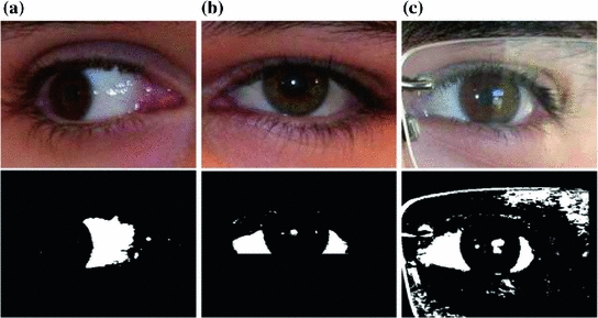
a Original, normalized image, b binary mask where ‘1’ represents pixels whose gradient modulus ( $\left| \nabla I(x,y)\right|$ ) is above 0.1, c binary mask with filled regions, and d binary mask only with regions of high intensity pixels

Fig. 5

Preliminary results identifying the “reflex region”: (top row) original images and (bottom row) binary Sclera masks. In (c) many classification errors are still present due to glasses lens and frame

Fig. 6

Results of the application of the 4 morphological operators described in Sect. 3.3 on the binary mask shown in Fig. 5c. a Opening with a circular element of radius 3. b Erosion with a circular element of radius 4. c Removal of elements with area of less than 4 pixels. d Dilation with a circular element of radius 7

Fig. 7

Two examples of segmented sclera regions

The center of the different regions are then used as seeds for a Watershed analysis [41] that allows us to obtain accurate edges for each region in the image. Different regions, accordingly to the gradient formulation, are then defined whenever a basin area is not significantly changing for consistent intensities variation (water filling approach [2, 46]).

3.4 Final Classification Step

The aforementioned algorithm provides no false negative regions but many false positives are present in images where ambiguous regions, due to glasses or contact lenses reflexes, are confused with sclera. Analyzing all the images included in the considered database, we observe that the true sclera region have only two possible configurations: (1) like a triangle with two extruded sides and one intruded (Fig. 7a) or, when the subject is looking up, (2) like two of the previous triangles, facing each other, and connected with a thin line on the bottom (Fig. 7b).

On the basis of these considerations, we decide to define a set of shape-based features that can be used to separate, among all the selected regions, those that represent real scleras. The vector is composed by the following elements (invariant to translations and rotations):

Region area in pixels;
Ratio between region area and its perimeter;
7 Hu invariant moments [15]. Concerning the seventh moment [15], we use its module since we do not want to distinguish mirror images.

The final region classifier is then based on a Support Vector Machine accordingly to the Cortes-Vapnik formulation [3]. Sclera and Non-Sclera regions are classified accordingly to:

$\begin{aligned} \hat{y}=sign\left( f(\mathbf {x})\right) , \end{aligned}$

(5)

where

$\begin{aligned} f(\mathbf {x})=\sum \limits _{i \in S} {\alpha _i y_i \varPhi \left( {{\mathbf {x}}_i }\right) \cdot } \varPhi \left( {\mathbf {x}} \right) + b = \sum \limits _{i \in S} {\alpha _i y_i \mathcal {K} \left( {{\mathbf {x}}_i ,{\mathbf {x}}} \right) } + b. \end{aligned}$

(6)

$\alpha _i$ are Lagrange multipliers, $$b$$

is a constant, $$S$$

are elements for which the relative multiplier $\alpha _i$ is non-null after optimization process and $\mathcal {K}$ is the non-linear kernel. In this case $\mathcal {K}$ is:

$\begin{aligned} \mathcal {K}(\mathbf {a},\mathbf {b})=\left( \mathbf {a} \cdot \mathbf {b} +1 \right) ^2. \end{aligned}$

(7)

This is a Quadratic Programming Problem that can be solved using optimization algorithms [14].

3.5 Results

Evaluating the segmentation results achieved over all the 250 chosen images (100 of them are also used for training) of the UBIRIS v.2 database, we obtain a 100 % recognition of closed eyes (no sclera pixels at all), 2 % false negative (with respect to the handmade segmented region) in the rare cases of very different brightness from left to right eye parts (due to a side illumination), and we also report a 1 % of false positive (with respect to the handmade segmented region) for particular glass-frames that locally resemble sclera regions.

4 Gaze Estimation

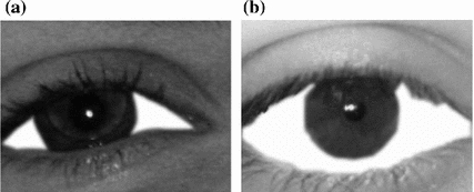
This Section, after a brief review of the state of the art methods that are well suited to our acquisition configuration, proposes a gaze-estimation technique. Normally, infrared (IR) light-emitting diodes (LEDs) are used in gaze estimation systems, as this light is not visible to humans and produces reflections on the cornea that are visible on the acquired images, called glints (see Fig. 8). When a beam light enters the cornea surface of a human eye, part of the light is reflected by the surface and part is refracted after traveling through the surface. The light which is reflected by the exterior cornea surface is called the first Purkinje image (see Fig. 8). Since the first Purkinje image is a result of specular reflection, observations at different directions will observe different images. Corneal reflections, together with the pupil center or the pupil contour or the limbus, are the eye features commonly used for gaze estimation. In particular, considering the WVU iris database acquisition setup, we estimate the gaze using corneal reflections (at least 2 are present in each image) and the pupil center (highlighted in Fig. 9b).

Fig. 8

Schematic diagram illustrating the geometry relationship between the point light source, the cornea, the first Purkinje image, and the camera. The bright spot in the image is the recorded first Purkinje image of an infrared LED (courtesy of Shih and Liu [33])

Most of the 3D model-based approaches employ 3D eye models and calibrated scenarios (calibrated cameras, light sources, and camera positions). Shih et al. [34] use the eye model proposed by Le Grand [17], where the shape of the cornea is assumed to be a portion of an imaginary sphere with center at $\mathbf {c}$ and radius R = 7.8 mm. The pupil is a circle on a plane distant ${\text {h}} = 4.2$ mm respect to the cornea center. The pupil and cornea centers define the optical axis (LoG). The cornea and the aqueous humor can be modeled as a convex spherical lens having uniform refraction index (as shown in Fig. 9a).

Fig. 9

a Structure of Le Grand’s simplified eye [17]. b Example of image of the WVU iris database, highlighting the features used for gaze estimation

The reflective properties of the cornea influence the position of the glint(s) in the image, while its refractive properties modify the pupil image. The pupil image is not the projection of the pupil, but the projection of the refracted pupil and this concept is fundamental also in the proposed iris correction method [40]. Figure 10 shows the 3D pupil inside the cornea and the pupil shape after refraction. The methods proposed by Villanueva et al. [40], Shih et al. [34] and Guestrin and Eizenman [12] are all based on the use of multiple light sources and one or more cameras for estimating the optical axis using pupil center and corneal reflections. In particular, we follow the latter method, even if the algorithms and the results of the aforementioned estimation processes are absolutely comparable. We work in the assumption that the light sources are modeled as point sources and the camera as a pin-hole camera [12]. Figure 11 presents a ray tracing diagram of the system and the eye for a single light and a single camera. We assume that the whole system is calibrated: the intrinsic camera parameters are known together with the positions of the LEDs respect to the camera (a plane mirror can be used to estimate each LED position as suggested by Shih and Liu [33]). All points are represented in a right-handed Cartesian world coordinate system aligned with the canonical camera reference system.

Fig. 10

3D model representing the real pupil and the virtual image of the pupil due to the refractive properties of the cornea (courtesy of Shih and Liu [33])