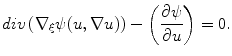
Fig. 1
Echocardiographic frame and its recognized Area
In the next part we focus the attention concerning the choice of the filter function for the edge-detection and the related applicability of the speed term formulation in the continuous model problem.
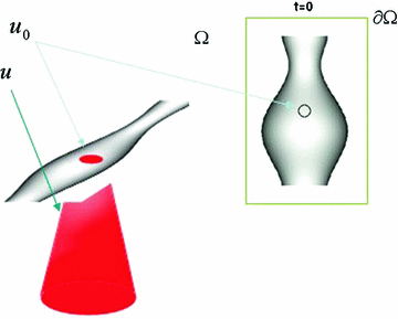
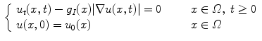
Fig. 2
Curve at isolevel at 
1.1 The Segmentation Problem
The aim of segmentation is to find a partition of an image into its costituent parts. For front evolution the  —
— standard model is adopted [1–3](Fig. 2).
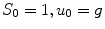
— standard model is adopted [1–3](Fig. 2).A curve in  can be represented as the zero-level line of a function in higher dimension. More precisely, let us suppose that there exists a function
  solution of the initial value problem:
which is the model of eikonal equation for front evolution for segmentation problem, typically involved in the detection for edges of objects contained in an image. We have to note that the evolving function  always remains a function as long as
  is smooth. So we choose a different expression for the speed terms in order to limit the loss of image definition of Gaussian smoothing and by new approach with functional minimization to preserve this property. For ours purposes we intend enough smooth a function
  , [4–12].
can be represented as the zero-level line of a function in higher dimension. More precisely, let us suppose that there exists a function solution of the initial value problem:(1)
always remains a function as long as is smooth. So we choose a different expression for the speed terms in order to limit the loss of image definition of Gaussian smoothing and by new approach with functional minimization to preserve this property. For ours purposes we intend enough smooth a function , [4–12].1.2 Edge-Detection
Given an image, in particular an echocardiographic image, we need to automatically detect the internal contour of object for clinical pourposes. We focus ours attention to a ventricular cavity. We consider a closed subset  of
of  having
  as the external edge of the rectangular image and being
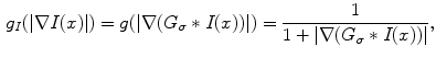
 ![$$I:\varOmega \rightarrow [0,1]$$](/wp-content/uploads/2016/03/A320009_1_En_16_Chapter_IEq12.gif) the brightness intensity. The “edge-detector” (detector of contours) for segmentation of the image is a positive real coefficient, which is dependent of
the brightness intensity. The “edge-detector” (detector of contours) for segmentation of the image is a positive real coefficient, which is dependent of  ’s gradient at every point of the curve [2, 13].
of having as the external edge of the rectangular image and being the brightness intensity. The “edge-detector” (detector of contours) for segmentation of the image is a positive real coefficient, which is dependent of ’s gradient at every point of the curve [2, 13].In particular, the model is represented by a filter function such that
 where
where
 decreasing with
  and
and
 such that
  and
and 
and and 1.3 Speed Choice for Image Processing
The speed term is dependent of the brightness intensity at every pixel and is directed along the outward normal, starting from an initial elliptic profile  centered in
centered in Insofar we define the composite function
where  *
*  is the convolution of the image
  with a regularizing operator
  whose algorithmic implementation we are going to explicit later. The operator
  is a filter that allows, by heat equation, to calculate the brightness-intensity gradient of the image in the presence of discontinuous data.
(2)
* is the convolution of the image with a regularizing operator whose algorithmic implementation we are going to explicit later. The operator is a filter that allows, by heat equation, to calculate the brightness-intensity gradient of the image in the presence of discontinuous data.The discretization of the problem is performed by building a rectangular lattice, which is made fine-grained according to image’s pixel definition. The curve is parametrized by means of a Lipschitz function. Therefore, the differential problem to be numerically solved will look as follows:
Considering the built-in function  such that
![$$\begin{aligned} \left\{ \begin{array}{ll} u_t - g_I (|\nabla I(x)|) | \nabla u | = 0 &{} \qquad x \in \varOmega \subset {\mathbb {R}}^2 \times [0,T]\\ u(x,0)=u_0(x) &{} \qquad x \in \varOmega \subset {\mathbb {R}}^2\\ \end{array} \right. \end{aligned}$$](/wp-content/uploads/2016/03/A320009_1_En_16_Chapter_Equ3.gif)
where T is the time horizon.
such that (3)
In the numerical tests the algorithm predicts a stop of the evolving curve at a threshold value  for the speed term, such that, if
  then the threshold parameter allows curve evolution to stop in the presence of different gradient values for the regularized image.
for the speed term, such that, if then the threshold parameter allows curve evolution to stop in the presence of different gradient values for the regularized image.2 New Approach to Regularize and Enhance Image
Analysis of images through variational methods finds application in a number of fields such as robotics, elaboration of satellite data, biomedical analysis and many other real-life cases. By segmentation is meant a search for constituent parts of an image, rather than an improving of its quality or characteristics. Our aim is to develop a criterium for enhancing movie frame in two possible ways by functional minimization. First, we adopt the M-S functional and its approximated form proposed by Ambrosio and Tortorelli [14] to regularize data frame for curve evolution method, instead of Gaussian regularization.
We call it “classic functional” since the function space the variational integral converges over contains functions that have the regularity needed for image gradient calculus. Second, we present a numerical scheme, where a time-dependent parameter is inserted, precisely in the second integral part of functional distinguished by a “time gradient”, for enhancing the internal moving parts of the object.
A detailed analytical treatment and a numerical scheme for minimization of the functional, which involves some delicate conjectures and refined mathematical steps, can be found in [15]. In the following section we recall in brief the essential formulation of the model problem used to regularize and enhance image. Other particular on numerical approximation and function space are explained in the next parts and in references. The reader can look up, for a complete review, the book by Morel and Solimini[16].
2.1 Ambrosio-Tortorelli Algorithm (’90)
This section refers to M-S algorithm for the approximation of  with a sequence
  of regular functionals defined on a Sobolev space. We focus our attention on the Ambrosio-Tortorelli approximation, which is among the most used in image analysis. In this particular approach, the set
  (or
(or  ) is replaced by an auxiliary variable
  (a function) which approximates the characteristic function
 If
If  minimizes the functional
  then the following result holds [14]:
 We gather from the problem of minimun related to the Ambrosio-Tortorelli functional, the Euler equations, than by an appropriate approximation will give us an algorithm for minimization.
with a sequence of regular functionals defined on a Sobolev space. We focus our attention on the Ambrosio-Tortorelli approximation, which is among the most used in image analysis. In this particular approach, the set (or ) is replaced by an auxiliary variable (a function) which approximates the characteristic function minimizes the functional then the following result holds [14]:When we apply Euler equation system, if  is chosen, an enough rapid continuation method will give good results even though contours are not well defined.
is chosen, an enough rapid continuation method will give good results even though contours are not well defined.2.2 Euler Equation of the Approximated Functional
Given
 the associated Euler equation is
 Using Neumann boundary conditions, we get:
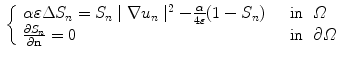
 Euler equation system for
  considering that the quadratic gradient
  is transformed into the Laplacian, looks as follows:
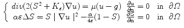 where the non linear terms
  and
and  cause the system to be non-linear and elliptic, with such a structure that, when
  is known, the first equation gets linear, while, if it is
  to be known, it is the second equation to be linear. This suggests the adoption of a two-stage iterative scheme. Where we fix the discrete step of convergence that is enough to give back a regularized image, enhanced in its content edge, as we present in the next section.
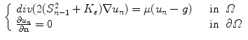
considering that the quadratic gradient is transformed into the Laplacian, looks as follows: and cause the system to be non-linear and elliptic, with such a structure that, when is known, the first equation gets linear, while, if it is to be known, it is the second equation to be linear. This suggests the adoption of a two-stage iterative scheme. Where we fix the discrete step of convergence that is enough to give back a regularized image, enhanced in its content edge, as we present in the next section.3 Approximation of the Models
We are going to describe, in this section, the numerical approximation of the models introduced above. In details, our aim is to present the semilagrangian scheme for curve evolution by numerical solution of eikonal equation. The standard mollifier is constructed by a Gaussian operator as a numerical scheme for heat eqution in two dimensions. The last section reports the procedure to build the approximation of the Mumford-Shah functional by Ambrosio-Tortorelli scheme.
3.1 Semi-Lagrangian Scheme for Eikonal Equation
Semi-Lagrangian (SL) schemes try to mimic the continuous behavior by constructing the solution at each grid point by back integration along the characteristic trajectory passing through the point and reconstructing the value at the foot of the trajectory by interpolation.
The numeric dependence of the domain contains its continuous dependence without any additional condition on  and
and  (space lattice is usually defined for finite differences as the pixel resolution of images). This allow a larger time steps than other schemes where the CFL condition has to be imposed for stability guaranty.
and (space lattice is usually defined for finite differences as the pixel resolution of images). This allow a larger time steps than other schemes where the CFL condition has to be imposed for stability guaranty.The numerical method for eq. (3) following the semilagrangian scheme by [17]. In our implementation we use a threshold value that has been chosen and discussed in a Master thesis [18].
We construct the protocol step of curve evolution by an oriented adaptation to medical application of HJPACK parallel OpenMp Fortran programming language.
3.2 Ambrosio-Tortorelli Approximation of the M-S Functional
The numerical scheme is made by dividing in two coupled parts with  and
and 
and At every step we calculate  for
for  solving a linear elliptic equation and, this way, we find
  from the second equation; this process is repeated for a fixed number of iterations.
for solving a linear elliptic equation and, this way, we find from the second equation; this process is repeated for a fixed number of iterations.3.2.1 System Discretization
We use a numerical scheme based on explicit finite differences, over the rectangle  with step
  ; this way we obtain
 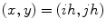 for
for  Reducing
  to a square of side 1 and taking
  discrete coordinates will become:
 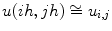 and
and 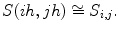
with step ; this way we obtain for Reducing to a square of side 1 and taking discrete coordinates will become: and We use an approximated scheme that is enough to enhancing little areas, characteristic of the echographic image. Some scheme for the Ambrosio-Tortorelli segmentation problem [19].
In order to determine the minimum of the functional we adopt the schema given, for a finite element, in [20] to a finite difference meshgrid through the following iterative scheme:
given a maximum number of iteration  and a tolerance ‘
 , then we construct:
 and
and  by solving:
From minimization theorem 3.1 Proposition 2.1 [20], it respectively follows that:
and a tolerance ‘, then we construct:
for find
find  , by solving:
by solving:
stop for .
.
 is a piecewise
  submanifolds of
  .
.For any ![$$n>1$$” src=”/wp-content/uploads/2016/03/A320009_1_En_16_Chapter_IEq68.gif”></SPAN> there exists <SPAN id=IEq69 class=InlineEquation><IMG alt=$$u_n$$ src=]() an
an  solution of the respective system which satisfy the bounds:
 Then we discretize the equations by finite differences.
solution of the respective system which satisfy the bounds:3.2.2 The Discreet Divergence
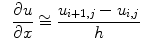
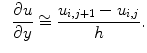
In a numerical scheme a function  can be approximated by finite difference, its first order variation on the
  direction is:
 and for
  direction is:
 The divergence of a function
  by second order of centered difference is given by
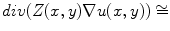

 where
where
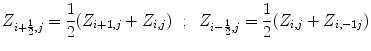
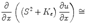
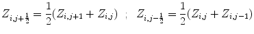 By applying to the system of Euler equation for the
  approximated item of the sequence of the Ambrosio-Tortorelli functional we obtain: the term
 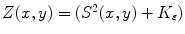 become by fixing every direction of the space, with
  neglected as in [19], we get: for x
![$$ \frac{1}{2h^2}\left[ (S^2 _{i+1,j} +S^2 _{i,j})(u_{i+1,j}-u_{i,j})+ (S^2 _{i,j} +S^2 _{i-1,j})(u_{i-1,j}-u_{i,j})\right] , $$](/wp-content/uploads/2016/03/A320009_1_En_16_Chapter_Equ26.gif) for y
for y
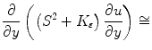
![$$ \frac{1}{2h^2}\left[ (S^2 _{i,j+1} +S^2 _{i,j})(u_{i,j+1}-u_{i,j})+ (S^2 _{i,j} +S^2 _{i,j-1})(u_{i,j-1}-u_{i,j})\right] . $$](/wp-content/uploads/2016/03/A320009_1_En_16_Chapter_Equ28.gif) In Image Processing the lattice has a spatial density which is equivalent to image resolution, so we use here finite differences with node resolution equal to the spatial grid-step, so the discretized equation will look as follows
In Image Processing the lattice has a spatial density which is equivalent to image resolution, so we use here finite differences with node resolution equal to the spatial grid-step, so the discretized equation will look as follows
 The discreet laplacian for a function u
 e-Slide in the e-Laboratory of Cytology: Where are We?
 Heritage and 3D Models
 of the Prognostic Relevance of Longitudinal Brain Atrophy in Post-traumatic Diffuse Axonal Injury Using Graph-Based MRI Segmentation Techniques
 Sampling and Reconstruction for Sparse Magnetic Resonance Imaging
 Image Segmentation: An Automatic Unsupervised Method
 Image Segmentation by Weighted Image Gradient Norm Terms Based on Local Histogram and Active Contours


can be approximated by finite difference, its first order variation on the direction is: direction is: by second order of centered difference is given by approximated item of the sequence of the Ambrosio-Tortorelli functional we obtain: the term become by fixing every direction of the space, with neglected as in [19], we get: for xRelated posts:
of the Prognostic Relevance of Longitudinal Brain Atrophy in Post-traumatic Diffuse Axonal Injury Using Graph-Based MRI Segmentation Techniques
Stay updated, free articles. Join our Telegram channel
Full access? Get Clinical Tree
