be an open and bounded set in  , and
, and ![$$I :\overline{\varOmega }\longrightarrow [0,L]$$](/wp-content/uploads/2016/03/A320009_1_En_13_Chapter_IEq3.gif) a scalar function, representing the observed grayscale input image. Based on the CV model [12, 15], the minimization problem to consider is
a scalar function, representing the observed grayscale input image. Based on the CV model [12, 15], the minimization problem to consider is

(1)
 is some feature input channel depending on the image, the vector
  with
with  and
and  are inside and outside unknown averages of
  , respectively. There are also
  and
and  . Vector
  has constant components that weight fitting terms.
2.1 The Proposed Feature Input Channels
Derivatives are a powerful tool for the extraction of features in images with texture (see e.g. [23]). Given a grayscale texture image displaying two different texture information, it is possible to discriminate between textures using the gradient vector and its norm [19].
Indeed, given a scalar image  , the new input channel is

where the lower subscript  in (2) means a smoothed version of the corresponding indexed function. Smoothing is done using a Gaussian function

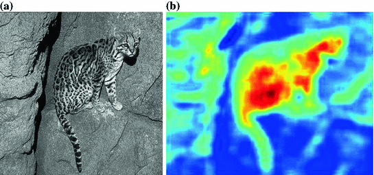
This new input channel  embodies different texture information. Nevertheless, it is not able to differentiate between similar scale textures in natural images, as can be seen in Fig. 1b. The input
  image, Fig. 1a, is an example of a natural image containing a texture object. In the image with comparable texture information both inside and outside the object of interest, the corresponding feature channel
  can not adequately distinguish the object itself, potentially leading to poor segmentation.
 , the new input channel is
(2)
 in (2) means a smoothed version of the corresponding indexed function. Smoothing is done using a Gaussian function
(3)
 embodies different texture information. Nevertheless, it is not able to differentiate between similar scale textures in natural images, as can be seen in Fig. 1b. The input
  image, Fig. 1a, is an example of a natural image containing a texture object. In the image with comparable texture information both inside and outside the object of interest, the corresponding feature channel
  can not adequately distinguish the object itself, potentially leading to poor segmentation.
To overcome this difficulty and to obtain a good input channel for the minimization approach (1), an image feature data descriptor is proposed using functions ( ) which contain information about image intensity. This will be combined with channel
  using the multiplication operation. The main idea about using
  is to help identify the edges between the texture object and the background. In this chapter, two different choices of the function
  are proposed.
 ) which contain information about image intensity. This will be combined with channel
  using the multiplication operation. The main idea about using
  is to help identify the edges between the texture object and the background. In this chapter, two different choices of the function
  are proposed.
 The first natural choice is
  (global information).
 Another choice for
  , called
  , is selected based on local cumulative distribution around a neighborhood of a given pixel, and then computing the total intensity given by the area under the local cumulative distribution curve (local information).
2.2 Weighted Gradient Based Fitting Terms I
Given a grayscale image ![$$I:\varOmega \rightarrow [0,L]$$](/wp-content/uploads/2016/03/A320009_1_En_13_Chapter_IEq28.gif) , using the Gaussian function (3) the following smoothed input channel is obtained:
, using the Gaussian function (3) the following smoothed input channel is obtained:

Then, the new fitting term is

It should be noticed that  involves computing three feature channels for each scale,
  and
and  , differentiating the proposed model from the Gabor filters [33, 36] for texture image segmentation. Gabor filters have the drawback of inducing a lot of redundancy feature channels. Other texture features involving image gradient were also considered by Brox et al. [7, 35]. They used the structure tensor notion defined by the matrix

![$$I:\varOmega \rightarrow [0,L]$$](/wp-content/uploads/2016/03/A320009_1_En_13_Chapter_IEq28.gif) , using the Gaussian function (3) the following smoothed input channel is obtained:
, using the Gaussian function (3) the following smoothed input channel is obtained:
(4)

(5)
 involves computing three feature channels for each scale,
  and
and  , differentiating the proposed model from the Gabor filters [33, 36] for texture image segmentation. Gabor filters have the drawback of inducing a lot of redundancy feature channels. Other texture features involving image gradient were also considered by Brox et al. [7, 35]. They used the structure tensor notion defined by the matrix
(6)
2.2.1 Color Extension
The proposed model can be extended to color images using the vector-value CV model extension [13]. For a color image  , where
  and
and  represent red, green and blue input channels, respectively, the new fitting terms are

 , where
  and
and  represent red, green and blue input channels, respectively, the new fitting terms are
(7)
2.3 Weighted Gradient Based Fitting Terms II
Another weighted gradient based fitting term is proposed herein using local histograms. Local histograms give a complete description of image intensity around each pixel and do not depend on regions [2, 11, 32]. For a given grayscale image ![$$I :\overline{\varOmega }\longrightarrow [0,L]$$](/wp-content/uploads/2016/03/A320009_1_En_13_Chapter_IEq35.gif) , let
, let  be the local region centered at a pixel
  with radius
  . The local histogram of a pixel
  and its corresponding cumulative distribution function for input channel
  are defined, respectively, by
 and
and
 for
for  . Then,
  is defined
 With
With  the total intensity weight within the neighborhood
  of
of  is obtained, in contrast with
  , which only gives the intensity value in
  . Together with the image gradient norm, the following input channel is considered:

with an associated fitting term
 The notion of local histogram for texture image segmentation has also been taken into account by Ni et al. [22, 32]. The current approach differs from previous work mainly because it does not use the Wasserstein distance in segmentation formulation.

![$$I :\overline{\varOmega }\longrightarrow [0,L]$$](/wp-content/uploads/2016/03/A320009_1_En_13_Chapter_IEq35.gif) , let
, let  be the local region centered at a pixel
  with radius
  . The local histogram of a pixel
  and its corresponding cumulative distribution function for input channel
  are defined, respectively, by

 . Then,
  is defined
 the total intensity weight within the neighborhood
  of
of  is obtained, in contrast with
  , which only gives the intensity value in
  . Together with the image gradient norm, the following input channel is considered:
(8)


Fig. 2
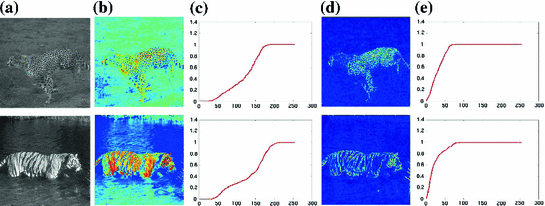
Local cumulative distribution functions of two images with different texture information. a Input images. b The scaled pixel-values of the input images showing the nature of texture present. c Corresponding local cumulative distribution functions inside the region of interest using  . d The scaled pixel-values of the gradient image. e Corresponding local cumulative distribution functions inside the region of interest in (d) using
 . d The scaled pixel-values of the gradient image. e Corresponding local cumulative distribution functions inside the region of interest in (d) using
Usually, two different types of texture images are found in natural images. The first are small scale textures corresponding to a lot of oscillations inside the main object, and the second consists of different flat regions given by large scale textures within the object of interest in the given image. Figure 2 shows two real images with different texture information. Figure 2a, shows  and
and  images, together with their corresponding pixel-valued image (scaled grayscale values) in Fig. 2b, and the computed local cumulative distribution function of the inner region of the main object to be segmented, Fig. 2c, with
  . As shown, the local cumulative distribution function for the
  has an almost convex shape over all the domain, whereas the
  image has a local cumulative distribution function which oscillates between convex and concave shapes. This is because the
  has a lot of different flat regions inside the body which can be considered as large scale textures. Then, the image gradient norm is used in the computation of local histograms in order to apply the weighted gradient fitting term approach. Figure 2d shows how the image gradient norm recovers oscillations patterns inside the
  image. Furthermore, Fig. 2e shows that local cumulative distribution functions corresponding to the image gradient norm have an almost single convex shape over the whole domain.
 and
and  images, together with their corresponding pixel-valued image (scaled grayscale values) in Fig. 2b, and the computed local cumulative distribution function of the inner region of the main object to be segmented, Fig. 2c, with
  . As shown, the local cumulative distribution function for the
  has an almost convex shape over all the domain, whereas the
  image has a local cumulative distribution function which oscillates between convex and concave shapes. This is because the
  has a lot of different flat regions inside the body which can be considered as large scale textures. Then, the image gradient norm is used in the computation of local histograms in order to apply the weighted gradient fitting term approach. Figure 2d shows how the image gradient norm recovers oscillations patterns inside the
  image. Furthermore, Fig. 2e shows that local cumulative distribution functions corresponding to the image gradient norm have an almost single convex shape over the whole domain.
2.3.1 Some Extensions
Extensions for the input channel (8) are listed below.
 The local histogram computation can also be applied to the image gradient norm instead of the original input image
  . That is,
  is considered together with the input channel
(9)

 By combining (8) and (9), another extension is defined with the data term
(10)
 .
. The previous extension can be applied to color images using RGB decomposition. For a texture color image
  , where
  and
and  represent red, green and blue input channels, respectively, the new fitting terms are
(11)
 and
and  .
.3 Numerical Solution for the Proposed Model
A two-step methodology is implemented for solving the proposed texture segmentation approach (1). In the first step,  is fixed and the minimization with respect to
  is computed. Then,
  is fixed and the minimization with respect to
  is performed. Although the functional
  is convex in
  , the minimization is carried out over a binary set. Following the same approach as in Chan et al. [12], it is proposed to use soft smooth membership function
 ![$$u\in [0,1]$$](/wp-content/uploads/2016/03/A320009_1_En_13_Chapter_IEq74.gif) . The new convex minimization problem is
. The new convex minimization problem is
![$$\begin{aligned} \begin{array}{lcl } \min \limits _{u\,\in \,[0,1]}G({\mathbf {c}},u), \end{array} \end{aligned}$$](/wp-content/uploads/2016/03/A320009_1_En_13_Chapter_Equ12.gif)
for which it is guaranteed the existence of a global minimizer. Moreover, if  is a minimizer of the convex relaxed problem (12), then for a.e.
 ![$$s\in [0,1]$$](/wp-content/uploads/2016/03/A320009_1_En_13_Chapter_IEq76.gif) , the function
, the function ![$$\hat{u}={1\!\!1}_{\{{\mathbf {x}}\,\in \,\varOmega \,:\,u({\mathbf {x}})> s\}}$$” src=”/wp-content/uploads/2016/03/A320009_1_En_13_Chapter_IEq77.gif”></SPAN> is a minimizer of the original binary problem (<SPAN class=InternalRef><A href=]() 1). The minimization of (12) can be efficiently solved using the dual minimization approach of the TV term [6, 10].
1). The minimization of (12) can be efficiently solved using the dual minimization approach of the TV term [6, 10].
 is fixed and the minimization with respect to
  is computed. Then,
  is fixed and the minimization with respect to
  is performed. Although the functional
  is convex in
  , the minimization is carried out over a binary set. Following the same approach as in Chan et al. [12], it is proposed to use soft smooth membership function
 ![$$u\in [0,1]$$](/wp-content/uploads/2016/03/A320009_1_En_13_Chapter_IEq74.gif) . The new convex minimization problem is
. The new convex minimization problem is![$$\begin{aligned} \begin{array}{lcl } \min \limits _{u\,\in \,[0,1]}G({\mathbf {c}},u), \end{array} \end{aligned}$$](/wp-content/uploads/2016/03/A320009_1_En_13_Chapter_Equ12.gif)
(12)
 is a minimizer of the convex relaxed problem (12), then for a.e.
 ![$$s\in [0,1]$$](/wp-content/uploads/2016/03/A320009_1_En_13_Chapter_IEq76.gif) , the function
, the function 3.1 Fast Dual Minimization
A fast numerical algorithm applying the methods in Aujol et al. [4] and Bresson et al. [6] is implemented for solving the minimization problem (12). First, it should be noted that solving the minimization problem (12) is equivalent to solve
![$$\begin{aligned} \min _{u\,\in \,[0,1]}\Bigg \{\tilde{G}({\mathbf {c}},u) =\int _{\varOmega }\,|\nabla u |\, {\mathrm {d}}{\mathbf {x}} +\sum _{i=1}^{n}\int _{\varOmega }\Big (\lambda _{i}^{in}r_{i}\big (c_{i}^{in},f_{i}(I)\big )- \lambda _{i}^{out}r_{i}\big (c_{i}^{out},f_{i}(I)\big )\Big )\,u\, {\mathrm {d}}{\mathbf {x}}\Bigg \}. \end{aligned}$$](/wp-content/uploads/2016/03/A320009_1_En_13_Chapter_Equ25.gif)


![$$\begin{aligned} \min _{u\,\in \,[0,1]}\Bigg \{\tilde{G}({\mathbf {c}},u) =\int _{\varOmega }\,|\nabla u |\, {\mathrm {d}}{\mathbf {x}} +\sum _{i=1}^{n}\int _{\varOmega }\Big (\lambda _{i}^{in}r_{i}\big (c_{i}^{in},f_{i}(I)\big )- \lambda _{i}^{out}r_{i}\big (c_{i}^{out},f_{i}(I)\big )\Big )\,u\, {\mathrm {d}}{\mathbf {x}}\Bigg \}. \end{aligned}$$](/wp-content/uploads/2016/03/A320009_1_En_13_Chapter_Equ25.gif)
Stay updated, free articles. Join our Telegram channel

Full access? Get Clinical Tree


