The use of biomarkers of microvascular structure and function from perfusion and permeability imaging is now well established in neuro-oncological research. There remain significant challenges to be overcome before these techniques and related biomarkers can find general clinical acceptance. Core to this is the standardization of acquisition and processing protocols for robust use across multiple clinical sites. The potential clinical benefits of these approaches are already becoming clear, particularly in the setting of novel antiangiogenic therapies. With an increasing body of evidence in the scientific literature, and with a steadily falling barrier to entry, the coming decade should see rapid developments in imaging biomarkers, and facilitate their transition into routine clinical practice.
Most current clinical CT and MR imaging systems are capable of acquiring images with high temporal and spatial resolution data. Improvements in entry-level MR imaging technology have allowed for routine clinical use of certain relatively complex imaging sequences previously restricted to research studies. Parallel developments at the vanguard of imaging technology have similarly facilitated the development and refinement of techniques aimed at quantification of dynamic physiological processes. Quantitative images of physiological parameters, such as blood flow, should, theoretically, be independent of the imaging modality or the individual system used. Although this is rarely the case in practice (discussed later), the paradigm of clinically acceptable quantitative imaging with sufficient repeatability and reproducibility represents a shift in the approach to radiologic investigations. Such imaging measures are designated as biomarkers: “characteristics that are objectively measured and evaluated as an indicator of a normal biologic processes or pathogenic processes or pharmacologic responses to therapeutic intervention.” The minimally invasive description of physiological and pathophysiological processes has clear use in screening, diagnosis, prognostication, and treatment monitoring. Examples of currently accepted biomarkers include circulating tumor markers, such as prostate-specific antigen and CA 125. The performance characteristics of any measurement under consideration as a biomarker are key. Sensitivity, specificity, repeatability, reproducibility, and logistics must be taken into consideration. Unfortunately, the development of imaging biomarkers is more complex than that of circulating biomarkers, and standardization is currently lacking. Analyzing the same data with a variety of the commercially available software can result in significant discrepancies and when considering additional variations in scanner age, make, model, software version, and acquisition parameters, standardization can seem even more challenging. Despite these issues, certain imaging biomarkers are now widely used in clinical trials and increasingly finding routine clinical use. Oncology is an area with intense interest in imaging biomarkers. Although histopathology remains the gold standard diagnostic and prognostic tool, it is, by definition, invasive, precludes true longitudinal follow-up, and is subject to significant sampling bias. Given the importance of angiogenesis in tumor development, imaging biomarkers able to characterize the vascular microenvironment within tissues have been the subject of extensive research, largely driven by the development of antiangiogenic and vascular targeting agents for cancer treatment. This article reviews the imaging biomarkers of microvascular structure and function in common use and describes their potential clinical use.
Potential microvascular imaging biomarkers for neuro-oncology
Tumor growth is dependent on angiogenesis with consequent development of tumoral neovasculature. The angiogenic neovasculature commonly exhibits increased endothelial permeability to medium- and large-sized molecules as a direct effect of cytokine stimulation, which can be rapidly reversed by inhibition of the angiogenic pathway. In tumors, neoangiogenesis commonly leads to the development of distorted vascular beds, characterized by an excessive proportion of blood vessels and abnormal blood vessel morphology and flow characteristics. The development of pertinent imaging biomarkers has consequently focused on the estimation of capillary endothelial permeability and methods to characterize vascular density, vascular tortuosity, and other morphologic abnormalities, which represent the cumulative effects of the unchecked angiogenic process. Blood flow within the tumor vasculature, for example, reflects the structure of the vascular bed and also is affected by interstitial pressure, the arterial input vessel hierarchy, and local arteriovenous pressure difference. Although the measurement of blood flow characteristics is often referred to in the literature as perfusion or perfusion-weighted imaging, a distinction must be made between these two distinct properties. Perfusion is the process by which blood flow through a tissue provides nutrition and removes metabolic by-products. Blood flow through a tissue, or voxel, can occur without contributing to capillary perfusion and high flow is not always metabolically useful. Notwithstanding this distinction, imaging techniques used to directly quantify perfusion include H 2 15 O positron emission tomography (PET) and xenon-enhanced CT. These techniques are considered gold standard measurements of perfusion because the tracers have a high transfer coefficient and their concentration in brain tissue can be considered entirely dependent on vascular concentration and flow. Their use is logistically limited and alternative methods to estimate perfusion or other components of regional blood flow are more commonly used. Delivery models of freely diffusible tracers also preclude determination of permeability characteristics, and other approaches, therefore, are required.
Imaging techniques for microvascular characterization
A detailed description of the range of imaging and image analysis techniques used to produce biomarkers of microvascular structure and function is beyond the scope of this article; interested readers are directed to recent comprehensive review articles. In practice, three generic approaches are in common use: (1) dynamic contrast-enhanced (DCE) imaging; (2) arterial spin labeling (ASL); and (3) vascular space occupancy (VASO) imaging.
An overview of each of these approaches is presented, highlighting those aspects of the techniques that enhance understanding of potential clinical applications.
DCE Imaging
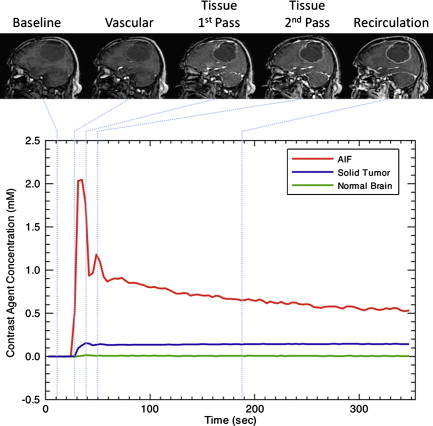
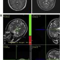
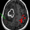
DCE techniques are the most commonly applied imaging techniques for the characterization of microvascular structure and function. Rapid, serial images are acquired during the administration of an intravenous contrast agent ( Fig. 1 ). These techniques can be applied to MR imaging (DCE–MRI) and CT (DCE-CT). The design of acquisition protocols is dependent on the image analysis approach chosen, which requires minimal standards of signal-to-noise ratio and temporal resolution. To achieve these goals, significant compromises may have to be made in spatial resolution or volume coverage.
The radiation doses of DCE-CT have restricted its application in drug trials, where repeated imaging is required. In clinical practice, however, DCE-CT is rapidly becoming a routine investigation, aided by the availability of modern CT equipment, the quantitative characteristics of the Hounsfield unit (or CT number), and the relationship between the attenuation and concentration of iodinated contrast media. DCE–MRI is ostensibly performed through the off-license use of clinically approved gadolinium-based contrast agents, although superparamagnetic and larger molecular weight agents are used in research. Two approaches are common, exploiting the susceptibility or relaxivity effects of the contrast media on the signal echo. It is worth mentioning at this point that the terminology in dynamic MR imaging can cause confusion. While DCE-MRI is a generic term for dynamic contrast-enhanced MR imaging, the terms dynamic relaxivity contrast enhanced (DRCE) and dynamic susceptibility contrast enhanced (DSCE) are not widely used to distinguish the two approaches. Instead, DCE-MRI is used to refer to T 1 -weighted relaxivity imaging, while dynamic susceptibility contrast (DSC)-MRI is used to refer to T2- or T2 -weighted susceptibility imaging. T 1 -weighted acquisitions are also frequently referred to as permeability imaging, while T2- or T2 -weighted techniques and CT are referred to as perfusion imaging due to their primary uses. As a result, perfusion weighted imaging (PWI) and perfusion CT (PCT) are sometimes used to refer to DSC-MRI and DCE-CT respectively. Furthermore, a dual echo MR approach which aims to provide susceptibility and relaxivity based measures in a single acquisition has been developed, and is usually prefixed by DE (dual echo). DSC–MR imaging has been widely applied in neuro-oncology, its acceptance promoted over CT by less onerous acquisition and postprocessing requirements. There are, however, several significant issues that should be appreciated: T2 -weighted acquisitions commonly have significant T 1 sensitivity, such that any contrast leakage produces artifactual elevations in the signal time course curve. Because the susceptibility effects manifest themselves as reductions in signal-echo intensity, relaxivity effects counter these and produce misleading signal changes. This is particularly problematic in tumors where blood-brain barrier breakdown has occurred. Acquisitions must, therefore, be designed to minimize the T 1 effect. The most common solution is the use of low flip angle gradient-echo sequences, which have low T 1 sensitivity.This has an adverse effect, however, on the signal-to-noise ratio. A full discussion of these issues is given in the article by Kassner and colleagues. Leakage correction can also be applied to minimise susceptibility effects by pre-dosing with gadolinium prior to acquisition—thereby saturating the extravascular extracellular space—by using software methods such as gamma variate fitting and baseline correction, or by a combination of all of these.
DCE-MRI utilises T 1 -weighted acquisitions in which relaxivity effects dominate. The major drawback of this approach is the difficulty in resolving the signal change effects resulting from intravascular contrast, contrast leakage, and contrast dispersion within the extravascular extracellular space (EES). Resolution of these and other issues has driven the development of a range of analysis approaches, which are discussed briefly.
Analysis of DCE Data
Early DCE–MRI studies used simple measurements of MR signal change over a specific time course or the change in morphology of the enhancement-time curve. Such parameters are unpredictably dependent on the scanning protocol and do not distinguish signal changes due to variations in blood flow ( F ), blood volume ( V ), and contrast leakage. Nonetheless, semiquantitative techniques provide clear clinical benefit in certain applications. To improve reproducibility and repeatability, the majority of more recent techniques involve the conversion of signal change to contrast agent concentration change over time, which is derived from the primary acquisitions. As alluded to previously, for CT data this is straightforward because the relationship between iodinated contrast agent concentration and the change in attenuation is linear. For DSC–MRI, the relation is nonlinear but easily calculated. The calculation of contrast concentration images from DCE–MRI data requires at least the accurate measurement of local tissue longitudinal relaxivity before contrast administration. As with all facets of MR imaging, the accuracy of T 1 measurement is a function of the imaging parameters used and can involve a trade-off with acquisition time on busy clinical scanners.
Contrast concentration time course data can be analyzed using a range of approaches, including pharmacokinetic models. The simplest of these is the initial area under the contrast concentration curve (IAUC). The IAUC is widely used in DCE analysis despite having little physiological specificity because it is highly reproducible and easy to calculate. The most commonly used approaches beyond this are designed to calculate physiological parameters, such as blood flow. The profusion of analysis approaches can be confusing, because many seem superficially to measure the same parameter (eg, flow) but do so in sometimes subtly distinct ways, such that results are not directly comparable.
As a result of the increasing adoption of disparate pharmacokinetic models, an attempt has been made to standardize the symbolic notation and nomenclature of the pertinent parameters. A selection of these is shown in Table 1 . The most complete of the extant approaches is the adiabatic tissue homogeneity model (AATH), which produces estimates of blood flow ( F ), capillary endothelial permeability surface area product per unit mass of tissue ( PS ), fractional blood-plasma volume ( v p ), and volume of extravascular, extracellular space (EES) per unit volume of tissue ( v e ). Although such physiological specificity is appealing, the demands on data quality in terms of signal-to-noise ratio and temporal resolution are highly restrictive. Consequently, simpler pharmacokinetic models, which are less specific but exhibit other desirable performance characteristics, are more widely used. Many of these combine the effects of F and PS into a single variable: the volume transfer constant between plasma and the EES ( K trans ). Although the usefulness of K trans is widely published, comparison of literature values is difficult due to the high dependence on the pharmacokinetic model and image acquisition parameters used. The result is that K trans estimates in different publications may represent different combinations of underlying physiological variables and, in addition, it is impossible to reliably determine which of these physiological characteristics dominate observed variations in K trans .
| Symbol | Short Name | Unit |
|---|---|---|
| Measured Quantities | ||
| C p | Tracer concentration in arterial blood plasma—arterial input function (MR imaging or CT) | mM |
| C a | Tracer concentration in arterial blood—arterial input function (PET) | kBq/mL |
| C t | Concentration of contrast agent at time, t, in every voxel | mM or kBq/mL |
| Estimated or predetermined quantities | ||
| MTT | Mean transit time | S |
| T | Capillary transit time | S |
| Calculated quantities | ||
| F | Blood flow | mL g −1 min −1 |
| CBF | Cerebral blood flow | mL g −1 min −1 |
| P | Total capillary-wall permeability | cm min −1 |
| PS | Permeability surface area product per unit mass of tissue | mL g −1 min −1 |
| E | Extraction fraction | None |
| K trans | Volume transfer constant between plasma and EES | Min −1 |
| K ep | Rate constant between EES and plasma | Min −1 |
| K i | Unidirectional influx constant | Min −1 |
| CBV | Cerebral blood volume | mL |
| v p | Fractional blood-plasma volume | None |
| V a | Fractional blood volume | None |
| v e | Volume of EES per unit volume tissue | None |
| V D | Volume of distribution of tracer | None |
| IAUC | Initial area under gadolinium contrast agent concentration–time curve | mM min |
Using DSC-MRI, calculation of cerebral blood flow (CBF) can be performed by comparison of the contrast concentration time course changes in a feeding artery (the arterial input function) with the changes in individual tissue voxels. The most common approach uses a deconvolution analysis to estimate CBF, cerebral blood volume (CBV), and mean transit time (MTT). Although widely used in ischemic cerebrovascular disease, this approach is less satisfactory in neuro-oncology due to regional variation in arterial flow characteristics within the tumor. Relative measures of CBV, CBF and MTT can be more simply derived from the DSC-MRI intensity-time curves based on the area under the curve—related to volume—and the time taken for the bolus to complete the first pass—related to MTT and therefore to CBF. First pass gamma-variate fitting is often used for this approach. For those individuals wishing further information on novel approaches to absolute flow measurement from DCE-MRI analysis, simple graphic analysis techniques to estimate flow based on the microsphere theorem are also used as described by Vallee and colleagues, although their usefulness in neuro-oncology is not yet clear.
Vascular Space Occupancy Imaging
In light of the technical problems associated with dynamic MR imaging, recent work has addressed the use of other tissue contrast mechanisms for examining tumor vascularity. VASO imaging is a T 1 -weighted technique, which differentiates blood from tissue to interrogate blood volume. It was originally used to calculate blood volume changes in experimental cortical functional magnetic resonance imaging (fMRI) but has since been applied to tumor imaging. While usually employing an inversion pulse to null intravascular T 1 -weighted signal, a simple approach to VASO, whereby T 1 -weighted images before and after contrast administration are subtracted and weighted, produces appropriate measures of relative (rCBV) or absolute cerebral blood volume in non-leaky tissues. In diseases such as tumors, where BBB breakdown has occurred, the signal increase reflects both blood volume and permeability. The values in normal tissue may be useful, however, for the calibration of CBV in other techniques.
Arterial Spin Labeling
ASL techniques exploit the differences in magnetization between static tissues and labeled blood water molecules produced by having a labeling slab or slice positioned over the feeding arterial supply. This produces pairs of flow-sensitized and control images in which the static tissue signals are identical but where the magnetization of the inflowing blood differs. The subtraction of control from labeled images yields a signal difference, which directly reflects local perfusion. The signal difference depends on many parameters including blood flow, the T 1 of blood and tissue, and the time taken for labelled blood to reach the imaging region (labeling delay). Signal differences can be as low as 1%, however conspicuity can be improved by employing inversion pulses to null the signal from static tissue before and after labelling. Despite the plethora of acronyms found in the ASL literature, there are two main classes of ASL techniques: continuous ASL (CASL) and pulsed ASL (PASL). In CASL, the supplying blood is continuously labeled below the imaging slab, until the tissue magnetization reaches a steady state. The PASL approach labels a thick slab of arterial blood at a single instance in time, and the imaging is performed after a sufficient delay to allow distribution in the tissue of interest. As with other dynamic imaging techniques, the final interpretation of ASL flow measurements depends on the labeling process and the subsequent analysis. Each has particular strengths and weaknesses and, therefore, lends itself to different imaging problems, although a compromise approach, known as pseudo- or pulsed CASL, has been developed, which may have benefits for more general use. Despite the challenges associated with ASL, it remains a desirable technique due to the absolute measures of cerebral blood flow it produces, and the fact that endogenous gadolinium contrast agents are not required.
Imaging techniques for microvascular characterization
A detailed description of the range of imaging and image analysis techniques used to produce biomarkers of microvascular structure and function is beyond the scope of this article; interested readers are directed to recent comprehensive review articles. In practice, three generic approaches are in common use: (1) dynamic contrast-enhanced (DCE) imaging; (2) arterial spin labeling (ASL); and (3) vascular space occupancy (VASO) imaging.
An overview of each of these approaches is presented, highlighting those aspects of the techniques that enhance understanding of potential clinical applications.
DCE Imaging
DCE techniques are the most commonly applied imaging techniques for the characterization of microvascular structure and function. Rapid, serial images are acquired during the administration of an intravenous contrast agent ( Fig. 1 ). These techniques can be applied to MR imaging (DCE–MRI) and CT (DCE-CT). The design of acquisition protocols is dependent on the image analysis approach chosen, which requires minimal standards of signal-to-noise ratio and temporal resolution. To achieve these goals, significant compromises may have to be made in spatial resolution or volume coverage.
The radiation doses of DCE-CT have restricted its application in drug trials, where repeated imaging is required. In clinical practice, however, DCE-CT is rapidly becoming a routine investigation, aided by the availability of modern CT equipment, the quantitative characteristics of the Hounsfield unit (or CT number), and the relationship between the attenuation and concentration of iodinated contrast media. DCE–MRI is ostensibly performed through the off-license use of clinically approved gadolinium-based contrast agents, although superparamagnetic and larger molecular weight agents are used in research. Two approaches are common, exploiting the susceptibility or relaxivity effects of the contrast media on the signal echo. It is worth mentioning at this point that the terminology in dynamic MR imaging can cause confusion. While DCE-MRI is a generic term for dynamic contrast-enhanced MR imaging, the terms dynamic relaxivity contrast enhanced (DRCE) and dynamic susceptibility contrast enhanced (DSCE) are not widely used to distinguish the two approaches. Instead, DCE-MRI is used to refer to T 1 -weighted relaxivity imaging, while dynamic susceptibility contrast (DSC)-MRI is used to refer to T2- or T2 -weighted susceptibility imaging. T 1 -weighted acquisitions are also frequently referred to as permeability imaging, while T2- or T2 -weighted techniques and CT are referred to as perfusion imaging due to their primary uses. As a result, perfusion weighted imaging (PWI) and perfusion CT (PCT) are sometimes used to refer to DSC-MRI and DCE-CT respectively. Furthermore, a dual echo MR approach which aims to provide susceptibility and relaxivity based measures in a single acquisition has been developed, and is usually prefixed by DE (dual echo). DSC–MR imaging has been widely applied in neuro-oncology, its acceptance promoted over CT by less onerous acquisition and postprocessing requirements. There are, however, several significant issues that should be appreciated: T2 -weighted acquisitions commonly have significant T 1 sensitivity, such that any contrast leakage produces artifactual elevations in the signal time course curve. Because the susceptibility effects manifest themselves as reductions in signal-echo intensity, relaxivity effects counter these and produce misleading signal changes. This is particularly problematic in tumors where blood-brain barrier breakdown has occurred. Acquisitions must, therefore, be designed to minimize the T 1 effect. The most common solution is the use of low flip angle gradient-echo sequences, which have low T 1 sensitivity.This has an adverse effect, however, on the signal-to-noise ratio. A full discussion of these issues is given in the article by Kassner and colleagues. Leakage correction can also be applied to minimise susceptibility effects by pre-dosing with gadolinium prior to acquisition—thereby saturating the extravascular extracellular space—by using software methods such as gamma variate fitting and baseline correction, or by a combination of all of these.
DCE-MRI utilises T 1 -weighted acquisitions in which relaxivity effects dominate. The major drawback of this approach is the difficulty in resolving the signal change effects resulting from intravascular contrast, contrast leakage, and contrast dispersion within the extravascular extracellular space (EES). Resolution of these and other issues has driven the development of a range of analysis approaches, which are discussed briefly.
Analysis of DCE Data
Early DCE–MRI studies used simple measurements of MR signal change over a specific time course or the change in morphology of the enhancement-time curve. Such parameters are unpredictably dependent on the scanning protocol and do not distinguish signal changes due to variations in blood flow ( F ), blood volume ( V ), and contrast leakage. Nonetheless, semiquantitative techniques provide clear clinical benefit in certain applications. To improve reproducibility and repeatability, the majority of more recent techniques involve the conversion of signal change to contrast agent concentration change over time, which is derived from the primary acquisitions. As alluded to previously, for CT data this is straightforward because the relationship between iodinated contrast agent concentration and the change in attenuation is linear. For DSC–MRI, the relation is nonlinear but easily calculated. The calculation of contrast concentration images from DCE–MRI data requires at least the accurate measurement of local tissue longitudinal relaxivity before contrast administration. As with all facets of MR imaging, the accuracy of T 1 measurement is a function of the imaging parameters used and can involve a trade-off with acquisition time on busy clinical scanners.
Contrast concentration time course data can be analyzed using a range of approaches, including pharmacokinetic models. The simplest of these is the initial area under the contrast concentration curve (IAUC). The IAUC is widely used in DCE analysis despite having little physiological specificity because it is highly reproducible and easy to calculate. The most commonly used approaches beyond this are designed to calculate physiological parameters, such as blood flow. The profusion of analysis approaches can be confusing, because many seem superficially to measure the same parameter (eg, flow) but do so in sometimes subtly distinct ways, such that results are not directly comparable.
As a result of the increasing adoption of disparate pharmacokinetic models, an attempt has been made to standardize the symbolic notation and nomenclature of the pertinent parameters. A selection of these is shown in Table 1 . The most complete of the extant approaches is the adiabatic tissue homogeneity model (AATH), which produces estimates of blood flow ( F ), capillary endothelial permeability surface area product per unit mass of tissue ( PS ), fractional blood-plasma volume ( v p ), and volume of extravascular, extracellular space (EES) per unit volume of tissue ( v e ). Although such physiological specificity is appealing, the demands on data quality in terms of signal-to-noise ratio and temporal resolution are highly restrictive. Consequently, simpler pharmacokinetic models, which are less specific but exhibit other desirable performance characteristics, are more widely used. Many of these combine the effects of F and PS into a single variable: the volume transfer constant between plasma and the EES ( K trans ). Although the usefulness of K trans is widely published, comparison of literature values is difficult due to the high dependence on the pharmacokinetic model and image acquisition parameters used. The result is that K trans estimates in different publications may represent different combinations of underlying physiological variables and, in addition, it is impossible to reliably determine which of these physiological characteristics dominate observed variations in K trans .
| Symbol | Short Name | Unit |
|---|---|---|
| Measured Quantities | ||
| C p | Tracer concentration in arterial blood plasma—arterial input function (MR imaging or CT) | mM |
| C a | Tracer concentration in arterial blood—arterial input function (PET) | kBq/mL |
| C t | Concentration of contrast agent at time, t, in every voxel | mM or kBq/mL |
| Estimated or predetermined quantities | ||
| MTT | Mean transit time | S |
| T | Capillary transit time | S |
| Calculated quantities | ||
| F | Blood flow | mL g −1 min −1 |
| CBF | Cerebral blood flow | mL g −1 min −1 |
| P | Total capillary-wall permeability | cm min −1 |
| PS | Permeability surface area product per unit mass of tissue | mL g −1 min −1 |
| E | Extraction fraction | None |
| K trans | Volume transfer constant between plasma and EES | Min −1 |
| K ep | Rate constant between EES and plasma | Min −1 |
| K i | Unidirectional influx constant | Min −1 |
| CBV | Cerebral blood volume | mL |
| v p | Fractional blood-plasma volume | None |
| V a | Fractional blood volume | None |
| v e | Volume of EES per unit volume tissue | None |
| V D | Volume of distribution of tracer | None |
| IAUC | Initial area under gadolinium contrast agent concentration–time curve | mM min |
Using DSC-MRI, calculation of cerebral blood flow (CBF) can be performed by comparison of the contrast concentration time course changes in a feeding artery (the arterial input function) with the changes in individual tissue voxels. The most common approach uses a deconvolution analysis to estimate CBF, cerebral blood volume (CBV), and mean transit time (MTT). Although widely used in ischemic cerebrovascular disease, this approach is less satisfactory in neuro-oncology due to regional variation in arterial flow characteristics within the tumor. Relative measures of CBV, CBF and MTT can be more simply derived from the DSC-MRI intensity-time curves based on the area under the curve—related to volume—and the time taken for the bolus to complete the first pass—related to MTT and therefore to CBF. First pass gamma-variate fitting is often used for this approach. For those individuals wishing further information on novel approaches to absolute flow measurement from DCE-MRI analysis, simple graphic analysis techniques to estimate flow based on the microsphere theorem are also used as described by Vallee and colleagues, although their usefulness in neuro-oncology is not yet clear.
Vascular Space Occupancy Imaging
In light of the technical problems associated with dynamic MR imaging, recent work has addressed the use of other tissue contrast mechanisms for examining tumor vascularity. VASO imaging is a T 1 -weighted technique, which differentiates blood from tissue to interrogate blood volume. It was originally used to calculate blood volume changes in experimental cortical functional magnetic resonance imaging (fMRI) but has since been applied to tumor imaging. While usually employing an inversion pulse to null intravascular T 1 -weighted signal, a simple approach to VASO, whereby T 1 -weighted images before and after contrast administration are subtracted and weighted, produces appropriate measures of relative (rCBV) or absolute cerebral blood volume in non-leaky tissues. In diseases such as tumors, where BBB breakdown has occurred, the signal increase reflects both blood volume and permeability. The values in normal tissue may be useful, however, for the calibration of CBV in other techniques.
Arterial Spin Labeling
ASL techniques exploit the differences in magnetization between static tissues and labeled blood water molecules produced by having a labeling slab or slice positioned over the feeding arterial supply. This produces pairs of flow-sensitized and control images in which the static tissue signals are identical but where the magnetization of the inflowing blood differs. The subtraction of control from labeled images yields a signal difference, which directly reflects local perfusion. The signal difference depends on many parameters including blood flow, the T 1 of blood and tissue, and the time taken for labelled blood to reach the imaging region (labeling delay). Signal differences can be as low as 1%, however conspicuity can be improved by employing inversion pulses to null the signal from static tissue before and after labelling. Despite the plethora of acronyms found in the ASL literature, there are two main classes of ASL techniques: continuous ASL (CASL) and pulsed ASL (PASL). In CASL, the supplying blood is continuously labeled below the imaging slab, until the tissue magnetization reaches a steady state. The PASL approach labels a thick slab of arterial blood at a single instance in time, and the imaging is performed after a sufficient delay to allow distribution in the tissue of interest. As with other dynamic imaging techniques, the final interpretation of ASL flow measurements depends on the labeling process and the subsequent analysis. Each has particular strengths and weaknesses and, therefore, lends itself to different imaging problems, although a compromise approach, known as pseudo- or pulsed CASL, has been developed, which may have benefits for more general use. Despite the challenges associated with ASL, it remains a desirable technique due to the absolute measures of cerebral blood flow it produces, and the fact that endogenous gadolinium contrast agents are not required.
Related posts:
 State-of-the-Art Pathology: New WHO Classification, Implications, and New Developments
 Molecular Tools: Biology, Prognosis, and Therapeutic Triage
 Advanced Imaging in Brain Tumor Surgery
 Novel Medical Therapeutics in Glioblastomas, Including Targeted Molecular Therapies, Current and Future Clinical Trials
 Clinical Trials in Brain Tumor Surgery
 Imaging of Brain Tumors: Functional Magnetic Resonance Imaging and Diffusion Tensor Imaging
Stay updated, free articles. Join our Telegram channel

Full access? Get Clinical Tree


