Guillaume DUHAMEL1,2, Olivier GIRARD1,2, Paulo LOUREIRO DE SOUSA3 and Lucas SOUSTELLE1,2 1 CRMBM, CNRS, Université Aix-Marseille, France 2 CEMEREM, AP-HM, Hôpital de la Timone, Marseille, France 3 ICUBE, CNRS, Université de Strasbourg, France Magnetic dipolar interaction is ubiquitous in MRI. The hydrogen nuclei (commonly called protons or simply spins, and are the focus of this chapter) have a quantum spin number equal to ½, which corresponds to an energy diagram with two distinct levels for a model of isolated spins in the presence of an external magnetic field B0. The Larmor frequency (i.e. the NMR resonance frequency, see Chapter 1) is determined by the difference between these two energy levels and is directly proportional to the value of the local magnetic field “seen” by the spins. At a microscopic scale, the spins behave like small magnets and create a characteristic magnetic field that affects their close neighbors (this is called magnetic dipolar coupling). This local magnetic field is superposed to the external magnetic field B0, with a consequent local modification of resonant frequency for close neighbors. This mechanism is the cause of the resonance line broadening (spectral, i.e. frequential, representation, of the NMR signal of the spins (see Chapter 9)) of the protons in macromolecules with restricted motion. This broadening is related to dipolar coupling and corresponds to a very rapid decay of the signal in the time domain with corresponding ultrashort transverse relaxation times T2 of the order of tens of microseconds (µs), in contrast to free-water protons which have a T2 of the order of tens of milliseconds (ms). In conventional MRI, reducing the echo time to durations shorter than a millisecond is generally not possible due to the presence of the magnetic field gradients required for the spatial encoding of the image (see Chapters 1 and 3). Macromolecules with restricted motion are thus invisible as their MRI signal decays too quickly to provide enough signal at the moment of the echo, contrarily to free water, which is easily detected via MRI. A typical example of macromolecules with these properties can be found in the myelin sheath of the central nervous system (Figure 8.1). This biological structure of primordial importance for brain functioning originates from the membrane of the oligodendrocytes that surround the axons in a very compact way. It carries out the task of electrical isolation of the axons and ensures good functioning of the nervous action potential. Contrary to other biological membranes, where lipids usually represent around 40% of the mass, myelin is very rich in lipids (cholesterol (40%), phospholipids (40%), and glycolipids (20%)) that represent ~75% of its mass. From the structural point of view, the compact wrapping of the membrane results in a multilayer organization of lipid bilayers in which the protons of the methylene groups (-CH2) of the long carbonate chains are spatially constrained and strongly restricted in their motion (Morell 2013), and thus they are characterized by extremely short T2 values. Since it is impossible to directly detect the signal of protons in macromolecules with ultrashort T2 using conventional MRI, novel techniques, that are the subject of this chapter, have been proposed. They can be classified into two categories: (1) magnetization transfer (MT) techniques and, in particular, inhomogeneous magnetization transfer (ihMT), which exploit the phenomena of exchanges between the populations of protons in macromolecules and the protons in free water in order to detect the presence of the former measuring the signal from the latter; (2) ultrashort echo time (UTE) techniques for which the spatial encoding of the image has been redesigned to reach sufficiently short echo times and thus to detect protons with T2 values shorter than a millisecond. The first part of this chapter presents the basics of the mechanisms leading to the dipolar broadening of resonance lines in MRI and helps us to understand the difference between the long relaxation times of protons in very mobile molecules (free water) and the very short ones of protons in macromolecules with restricted motion (usually called semi-solid) such as the lipid membranes that form myelin. The second part of the chapter describes the details of the ihMT and UTE techniques for acquiring images of biological tissues with ultrashort T2 values, with an emphasis on myelin imaging. Finally, some perspectives and conclusions will be presented. Figure 8.1. Schematic representation of the myelin sheath formed by a very compact wrapping of lipid bilayers (a hydrophilic head and a long hydrophobic carbonate chain (-CH2)) around the axons. The magnetic dipolar interaction is the main cause of resonance line broadening in proton NMR (Slichter 1990; Levitt 2008). A classical representation (valid for ½ spins in most situations) consists of considering each hydrogen nucleus as a small magnet (or magnetic dipole containing a north pole and a south pole) that generates a magnetic field in its close vicinity, similar to the lines of the Earth’s magnetic field that make a loop to connect the two poles (Figure 8.2). The dipolar interaction is defined as the interaction of these local magnetic fields induced by two neighboring spins, that is, between two magnetic dipoles. By definition, this interaction is mutual: it affects both nuclei and propagates in space without requiring direct physical contact between the two. In practice, for high values of static magnetic field B0 (of the order of 1 T, i.e. more than 10,000 times the value of the Earth’s magnetic field, about 50 µT), only the longitudinal component (i.e. the one aligned with B0) of these local dipolar fields is of interest, due to the very rapid precession of the spins around the B0 field that lead to an average zero value for the transverse components of the local dipolar magnetic fields. This is a secular approximation that is commonly used in NMR. A rigorous treatment of the dipolar interaction in NMR is based on the quantum mechanical formalism of the spin’s Hamiltonian, which represents the energy of the interactions (e.g. with an external B0 field, between the spins, etc.) that occur in the considered spin system. This formalism is often quite complex to comprehend1, and the treatment differs depending on whether the considered nuclei are of the same kind (homonuclear case) or different kinds (heteronuclear case). The main difference stems from the existence of an additional term in the dipolar Hamiltonian for the homonuclear case, corresponding to an iso-energetic exchange of magnetization between the coupled spins, that is, this exchange does not require any energy contribution from the environment (commonly called the “lattice”). This is typically the case of flip-flop, a term used to designate the transition of a spin from its up state to its down state simultaneously to the opposite transition of the neighbor spin from its down state to its up state. In the homonuclear case, this double transition is iso-energetic (it does not cost anything from an energy point of view, which is not the case of heteronuclear spins). Therefore, it enables efficient MT between the spins coupled via dipolar interaction and it is, hence, the root of spin diffusion (which is more efficient the stronger the magnetic coupling) that enables the exchange of magnetization within a sample without any physical or chemical exchange of matter. This is an important phenomenon of MT in macromolecules with restricted motion (that present residual nonzero dipolar coupling (see section 8.3)), such as the lipid chains contained in biological membranes (van Zijl et al. 2003; Chen et al. 2006; Malyarenko et al. 2014). In the case of two magnetically coupled 1H protons that we consider here, the dipolar Hamiltonian is directly proportional to the secular dipolar coupling Dsec given by: where µ0 is the magnetic permeability of vacuum, ?H is the gyromagnetic ratio of the proton, ℏ is the reduced Planck’s constant, r is the distance between the two protons, and ? is the angle obtained by the vector that connects the two spins and the static magnetic field B0. ?sec is expressed in radians per second. It can be noted that the dipolar coupling strength decreases as a function of the inverse of the distance between the two nuclei to the power of three, and varies with the orientation of the internuclear vector with respect to the external magnetic field. At the “magic angle” ? ≅ 54.74° (value of θ for which 3 cos² ? = 1), the effect of the dipolar coupling is zero, although the nuclei are magnetically coupled. To give an order of magnitude, let us consider two protons located at 0.2 nm from one another (order of magnitude of the distance between the two protons of a water molecule, for example) and aligned with the magnetic field B0 (? = 0°, such that (3 cos² ? −1)/2 = 1). In such a case, the secular dipolar coupling is of the order of 15 kHz (expressed here in Hz for direct comparison with the Larmor frequency, of the order of 64 MHz for a field of 1.5 T). In a heterogeneous sample rich in protons, as is the case of biological tissues, there is a multitude of molecules and possible dipolar couplings between the different protons (Calucci et al. 2009). The latter can take place between protons of the same molecule (intramolecular) or between two different molecules (intermolecular). The intramolecular couplings are generally stronger due to the rapid decay of the dipolar coupling with the distance. First, let us consider the simplified case of purely static nuclei (the spins are motionless). A dipolar coupling constant could be calculated for all pairs of hydrogen nuclei and, hence, the local magnetic field perceived by each proton could be obtained. Due to the multitude of interaction distances and possible orientations within the nuclei pairs, a quasi-continuum of dipolar coupling values is expected, with an almost continuous distribution of the resonance frequency values that are intrinsic to each proton in the medium. The corresponding NMR line could then be calculated simply by integrating (i.e. summing up) the spectra of all of the protons contributing to the NMR signal. Although this mental exercise is almost impossible to perform in practice because of the too-high number of protons and couplings, intuitively, we can understand that the width of the obtained line for such a sample (a static one, as a reminder) would be of the order of magnitude of the strongest dipolar coupling values, that is, tens of kHz. This phenomenon is called the dipolar broadening of the resonance lines. However, the spins are not static, but in motion because of the thermal oscillations in the medium, and these motions will also affect the line width. Figure 8.2. Illustration of the concepts of dipolar broadening resonance line (a) and complete (b) and partial (c) motional averaging. When the spins are in motion, they do not experience the same value of magnetic field induced by their close neighbors over time, and they are sensitive to its average value over time. Different types of molecular motion can be distinguished: the motion that occurs internally to each molecule, the translational diffusion of the molecules, or the rotation of the molecules around themselves when they are free (see Levitt 2008; see also in particular section 8.6). These motions may be rapid or slow depending on the considered medium (e.g. the viscosity of a fluid changes the speed of the molecules’ displacement or rotation around themselves). From a formal point of view, a correlation time (?c) can be associated with each type of movement to quantify the time limit when the dipolar Hamiltonian is no longer correlated with its initial value since it has significantly evolved over time due to the motion. The fastest motion is the determining factor of the motional averaging in dipolar interactions. The more the motion is rapid, the shorter the associated correlation time and the stronger the averaging effects. In the case of free water (or isotropic liquid2), the correlation time of translational diffusion and molecular rotations is of the order of 10-12 s (Calucci et al. 2009). All of the molecular orientations have the same probability over time, hence the average dipolar Hamiltonian (that describes the average local dipolar field) is zero because the integral of the function (3 cos² ? − 1) for all of the possible orientations equals 0. Therefore, although a strong dipolar coupling between the two water protons exists in the static case, it does not have any effect on the observed resonance frequency for each proton in the case of free water and the resonance line is very thin, typically of the order of a few Hz. The line width is then representative of the pure transverse relaxation phenomena related to the fluctuations of the surrounding dipolar fields (T2 relaxation) or the non-uniformity of the B0 field, which can be related to an imperfect design of the MRI magnet or magnetic susceptibility effects (T2* relaxation contributions). In the case of macromolecules with constrained motion (e.g. myelin lipid chains), several couplings exist between protons but, in this case, the restricted molecular mobility hinders some of the possible orientations. The value of the average dipolar field perceived by the spins corresponds in such a case to the average of the dipolar field over all possible orientations of the molecule. In this case, the term residual dipolar coupling (RDC) is employed to describe the value of the dipolar coupling that remains after the time averaging due to motion. The RDC is weaker than the coupling obtained in the static case. It is relatively weak in the case of anisotropic liquids but can be strong (of the order of kHz) for non-mobile macromolecules or semi-solids that are present3 in biological tissues. In such cases, the line width is a combination of the transverse relaxation phenomena related to the fluctuations of the local dipolar fields and dipolar broadening effects induced by the residual component of the dipolar interaction. Often, a unique value of T2 (inversely proportional to the line width) is used, typically equal to a few tens of microseconds for semi-solid macromolecules in biological tissues. The RDC observed in such motion-restricted macromolecules is the basis of the dipolar order, that is, polarization of coupled spins in the local dipolar field produced by their close neighbors. This dipolar order is particularly relevant for ihMT imaging as we will see in this chapter. Quite often, a simplified biophysical model composed of two separate compartments is used in MRI to describe biological tissues. The first compartment describes the magnetization of liquid protons (i.e. mobile protons) and the second represents the magnetization of the so-called semi-solid protons (i.e. protons with restricted motion, such as those in the macromolecules composing the myelin). These two compartments are supposed to exchange energy since there are physiochemical phenomena, such as chemical exchange of protons or cross-relaxation, enabling magnetization to be transferred from one compartment to another. While the liquid compartment can be described by the so-called Zeeman magnetization (the classical concept of macroscopic nuclear magnetization in NMR), the semi-solid compartment (that differs from the other due to the existence of a nonzero RDC) requires considering two degrees of freedom for describing the distribution of energy levels populations of the corresponding system of spins. In this way, in addition to the Zeeman magnetization that corresponds to the polarization of the spins in the external magnetic field B0, another type of magnetization coexists, called the dipolar order, which corresponds to the polarization of the spins in the local dipolar fields created by their neighbors. Figure 8.3. Biophysical model of biological tissue subjected to an RF saturation pulse. The effects of an MRI scan during which a saturation radiofrequency (RF) pulse is applied to the biological tissue can be modeled using the Bloch equations4 modified to take into account the MT (Henkelman et al. 1993) and the theory of RF saturation in solids, initially developed by Provotorov (1962) and later reinterpreted and made widely popular by Goldman (1970). This theory considers the dipolar order (Figure 8.3) and describes the coupling of the magnetization’s degrees of freedom of the semi-solid protons compartment, the Zeeman magnetization (MZB), and the dipolar order (β) under the effect of RF saturation off-resonance at a frequency Δ (the term single frequency RF saturation is employed in this case). Thus, a system of coupled differential equations [8.2] (equations of Bloch–Provotorov) describing the evolution of the magnetizations MZA, MZB and β is obtained: T1A, T1B and T1D correspond to the longitudinal relaxation constant of the Zeeman magnetization of the liquid and semi-solid compartments and of the dipolar order, respectively. The terms RrfA,B = πω12gA,B(2πΔ) correspond to the rate of RF saturation of the liquid and semi-solid compartments induced by an RF pulse of intensity ω1 (expressed in rad/s5) and of a frequency offset Δ, where gA and gB correspond to the normalized absorption lines associated with the liquid (Lorentzian line shape) and semi-solid compartment (usually assumed to have a super-Lorentzian shape) (Morrison et al. 1995). D corresponds to the local dipolar field that can be calculated using the second moment of gB. Finally, R is the exchange constant of the MT between the liquid and semi-solid compartments. Two important features can be observed from the system of equations [8.2]: (i) the Zeeman magnetization of the semi-solid compartment (MZB) and the dipolar order (β) are decoupled in the absence of RF saturation (RrfB = 0) or when the pulse is played on resonance (Δ = 0); (ii) the RF saturation acts on MZB in two opposed ways, promoting its attenuation (–RrfBMZB term) as well as its recovery by means of the inflow from dipolar order (+2πΔRrfBβ term). Besides, if the system of spins is exposed to saturation with a total RF power ω12 that is simultaneously split into two symmetric saturation frequencies +Δ and –Δ (symmetric dual RF saturation) then, using the full expression of RrfB at the frequencies + Δ and – Δ, the Provotorov equations can be rewritten as: The symmetry hypothesis for the line shape of the semi-solid pool6 (gB(2πΔ) = gB (–2πΔ)) allows the system of equations [8.3] to be simplified such that the Bloch-Provotorov equations describing the evolution of the system of spins subjected to symmetric dual RF saturation are reduced to:
8
Imaging of Dipolar Interactions in Biological Tissues: ihMT and UTE
8.1. Introduction

8.2. Origins of ultrashort T2
8.2.1. Dipolar coupling in NMR

8.2.2. Dipolar resonance line broadening

8.2.3. Motional averaging
8.3. Imaging of the inhomogeneous magnetization transfer
8.3.1. Dipolar order and radiofrequency saturation


Related posts:


Stay updated, free articles. Join our Telegram channel

Full access? Get Clinical Tree


