(1)
Amersham, Buckinghamshire, UK
1.1 Introduction
1.2.1 Introduction
1.2.2 The Standard Model
1.2.4 Cathode Rays
1.2.5 α- and β-Particles
1.2.7 Protons
1.2.9 π-Mesons
1.3.1 Introduction
1.4 Applications
1.4.2 Monte Carlo Simulations
1.4.3 Non-medical
1.4.4 Medical
Abstract
This chapter provides an historical overview of non-radiative interactions of charged particles with matter.
1.1 Introduction
This chapter introduces the charged particles and their applications that are relevant to the uses of ionising radiation in diagnostic and therapeutic medicine. This will provide the background of the variety of applications of the theories of charged particle energy loss that are developed in the book. The chapter is divided into three sections following this Introduction. The first reviews the physical characteristics of these charged particles and their interactions and the histories of their discoveries which were dependent upon the detection of the transfer of kinetic energy to matter. The next reviews the early history of the development of theories describing this transfer, and the third section reviews the applications of these theories.
1.2 History and Discovery
1.2.1 Introduction
The organisation of a discussion of the history of the science of the interactions of charged particles with matter is surprisingly tricky. A simple chronological approach has the benefit in that it can perhaps elucidate the development of thought and experiment over time with the gaining of new knowledge and techniques. Yet it can suffer from those cases where either the theoretical explanation of an experimental result or the experimental validation of a theoretical prediction is separated considerably in time and can thus yield incoherence and complication in explanation and association. Similarly, the sharp division of the discussion into two components, those of theory and of experiment, can suffer from the same lack of coherence that chronology can offer. The approach taken here is to isolate the discussion in a manner so as to link chronology, theory and experiment together in as coherent a manner as possible. Hence, the introduction and review of the history of charged particle interactions with matter will be based upon particles with applications in medicine: cathode rays (electrons), α- and β-particles, internal conversion and Auger electrons, protons, heavy ions (in their initial presentation in the form of fission fragments), π−-mesons and the neutral indirectly ionising particles, photons and neutrons, which generate secondary fluxes of charged particles through interactions with the atoms of the medium. Clearly these are not all of the possible charged particles that could be considered, but are reflective of those that are associated with diagnostic and therapeutic medicine. This will follow a scientific current which will be roughly parallel to the chronology and the developments of theory and experiment. Congruity of the three specifications will not be complete as this will be impossible to achieve. However, it will provide, it is hoped, an appreciation of how our understanding of how charged particles interact with matter in discovery and experiment evolved.
While the genesis of the modern science and engineering of charged particle interactions with matter lies within the past 150 years, the general problem of the rate at which a moving object loses energy as it passes through a resistive medium has long been of practical interest. Perhaps the earliest modern development can be traced back to Book II of The Principia in which Newton (1687) described mathematically the resistance felt by objects moving through a fluid. Other investigators of this field, which evolved into fluid dynamics and aerodynamics, included Euler, d’Alembert and Bernoulli. Of peculiar interest to us is the treatise published by Robins (1742) on the kinematics of artillery and firearm projectiles through air, in which he described his invention of the ballistic pendulum as a means of measuring the velocity of a projectile. Robins wrote, … that if a globe sets out in a resisting medium with a velocity much exceeding that with which the particles of the medium would rush into a void space … the resistance of this medium to the globe will be … in proportion to its velocity. We may further conclude, that the resisting power of the medium will gradually diminish, as the velocity of the globe decreases…, a conjecture that could be considered prescient of the theory of a charged particle moving through a Fermi gas of electrons.
However, our interest will lie in more recent times, primarily in those following the triad of the years of 1895, 1896 and 1897, the years during which x-rays, radioactivity and the nature of the electron were discovered – results which each culminated in the awarding to the discoverers of the then newly presented Nobel Prize in Physics. But before we provide the historical foundations to the medical applications of the theory of charged particle interactions with matter described in this book, we first review the modern understanding of the constitution and organisation of these particles.
1.2.2 The Standard Model
“Who ordered that?”
II Rabi on the announcement of the discovery of the muon
As the intent of this book is to present, within the context of medical applications, the means by which moving charged particles interact with matter and yield a radiation absorbed dose, it is appropriate that we first review the nature of these particles, their compositions and their properties as described by the Standard Model. This model reflects our current understanding of nature and three of its four known forces (electromagnetic, weak and strong), and it represents one of the great pinnacles of physics and intellectual development in the latter part of the twentieth century. These four known forces have widely differing levels of magnitude or ‘strength’. These are reflected in Table 1.1.
Table 1.1
The four known forces of nature
Force | Mediating boson | Relative magnitude | Range of interaction |
|---|---|---|---|
Strong | Gluon | 1 | 1 fm |
Electromagnetic | Photon | 1/137 | ∞ |
Weak | W ±, Z 0 | 10−13 | 10−3 fm |
Gravity | Graviton | 10−38 | ∞ |
The periodicity of Mendeleev’s periodic table of the elements can be explained on the basis of systematic groupings of only three particles required to form atoms – protons, neutrons and electrons. An analogous situation requiring the simplification of complexity through the introduction of systematic arrangements of fundamental particles arose in the 1940s and 1950s with the discoveries of copious particles which required a similarly systematic means of explanation. From analyses of the systematics of the physical attributes of these particles (such as mass, charge, intrinsic spin, isotopic spin, lifetime), the Standard Model has evolved as a means of describing these particles.1
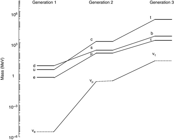
The Standard Model considers known matter to be made up of 12 elementary particles (and their antimatter partners) which are divided over three generations. Figure 1.1 shows the rest mass distribution of these particles. Each are fermions as they each have an intrinsic spin of ½ (in fundamental units of the reduced Planck constant,  ), making them subject to Fermi–Dirac statistics and the Pauli exclusion principle. Of the four particles assigned to each generation, the two with the greater masses are the quarks (the name having been coined by Murray Gell-Mann and derived from a quotation in Joyce’s Finnegan’s Wake, ‘Three quarks for Muster Mark’) and two are leptons (from the Greek λεπτοζ or leptos, meaning ‘small and thin’). The quarks have a unique quantum entity associated with them, that of flavour, and the states of the flavour quantum number are up (u), down (d), charm (c), strange (s), top (t) and bottom (b),2 with two flavours being assigned to each generation. Similarly, a pair of leptons is assigned to each generation, one which carries an electric charge (the electron (e), the μ-meson or muon (μ) and the tau lepton (τ)) and an electrically neutral neutrino that is associated with the charged lepton of that generation (i.e. the neutrino has a lepton flavour). The neutrino has, until recent times, been considered as having zero mass. Experimental evidence, however, has established a non-zero mass, the existence of which is reflected by neutrino oscillations in which neutrinos can change from one lepton flavour to another.
), making them subject to Fermi–Dirac statistics and the Pauli exclusion principle. Of the four particles assigned to each generation, the two with the greater masses are the quarks (the name having been coined by Murray Gell-Mann and derived from a quotation in Joyce’s Finnegan’s Wake, ‘Three quarks for Muster Mark’) and two are leptons (from the Greek λεπτοζ or leptos, meaning ‘small and thin’). The quarks have a unique quantum entity associated with them, that of flavour, and the states of the flavour quantum number are up (u), down (d), charm (c), strange (s), top (t) and bottom (b),2 with two flavours being assigned to each generation. Similarly, a pair of leptons is assigned to each generation, one which carries an electric charge (the electron (e), the μ-meson or muon (μ) and the tau lepton (τ)) and an electrically neutral neutrino that is associated with the charged lepton of that generation (i.e. the neutrino has a lepton flavour). The neutrino has, until recent times, been considered as having zero mass. Experimental evidence, however, has established a non-zero mass, the existence of which is reflected by neutrino oscillations in which neutrinos can change from one lepton flavour to another.Fig. 1.1
The Standard Model of the known elementary particles. Each generation contains a pair of quarks and a pair of leptons, one of which is the electrically neutral neutrino. The neutrino masses shown are the current estimates of their upper limits
With the exception of the neutrinos, all of the fermions carry an electric charge. The quarks have fractional charge (e.g. the up quark carries the charge  and the down quark carries the charge
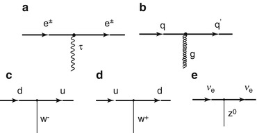
  ), whereas the charged leptons have an integral charge, ± 1e. Of course, the antiparticle counterparts carry the opposite electric charge. As the quarks are subject to the strong force, they, unlike the leptons, carry the additional quantum number of colour which has been assigned as the three states of red, green and blue. While only the quarks are subject to the strong force, all of the elementary particles of Fig. 1.1 are subject to the weak force,3 and all of the charged particles are subject to the electromagnetic force. The interactions via the three forces are mediated through bosons as shown in Fig. 1.2. Bosons have zero or integral spin (in units of
  ) and are thus described by Bose–Einstein statistics for which the Pauli exclusion principle is not applicable.
and the down quark carries the charge ), whereas the charged leptons have an integral charge, ± 1e. Of course, the antiparticle counterparts carry the opposite electric charge. As the quarks are subject to the strong force, they, unlike the leptons, carry the additional quantum number of colour which has been assigned as the three states of red, green and blue. While only the quarks are subject to the strong force, all of the elementary particles of Fig. 1.1 are subject to the weak force,3 and all of the charged particles are subject to the electromagnetic force. The interactions via the three forces are mediated through bosons as shown in Fig. 1.2. Bosons have zero or integral spin (in units of ) and are thus described by Bose–Einstein statistics for which the Pauli exclusion principle is not applicable.Fig. 1.2
Feynman diagrams of electromagnetic, strong and weak interaction vertices. (a) The charged electron/positron interacts with another charged particle through the mediation of a photon; (b) the strong force that a quark is subject to is mediated by a gluon; (c) and (d) the weak force-associated flavour changes of a quark are due to the exchange of the W − boson with the appropriate electric charge; and (e) the neutrino interacts weakly through the exchange of the neutral Z 0 boson. Charged particle energy loss is mediated through the electromagnetic process (a)
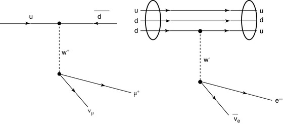
Quarks have not been detected as separate and individual entities, and all experimental evidence to date is that they form composite colour-neutral4 particles known as hadrons (from the Greek αδροζ or hadrós, meaning ‘thick’). A quark–antiquark pair forms a meson which has integral spin due to the coupling of their intrinsic spin-½ and any integral orbital angular momentum between the pair. For example, the positively charged π-meson consists of an up and an anti-down quark in the s state (i.e. with zero orbital angular momentum). Mesons are physically unstable and decay through weak interactions via the W ± and Z 0 intermediate vector bosons.5 , 6 The π+ consists of an up and anti-down quark pair and decays as  , mediated through a W + boson as shown in Fig. 1.3.
, mediated through a W + boson as shown in Fig. 1.3.Fig. 1.3
Feynman diagrams of the π + → μ + + ν μ decay and the β-decay of a neutron to a proton. The former decay is a weak process where the up and anti-down quarks of the pion annihilate to form a W + boson which then decays to create a positively charged muon and a neutrino. In the latter decay, a down quark transits to an up quark through the emission of a W − boson which subsequently decays to create an electron and an electron antineutrino
A quark triplet forms a baryon (from the Greek βαρυζ or barys, meaning ‘heavy’). For example, the proton consists of two up quarks and one anti-down quark and the neutron consists of two down quarks and one anti-up quark. As with the mesons, the baryons are colour neutral (e.g. consist of a red quark, a green quark and a blue quark so that the net combination of colours cancel with the result being referred to as ‘white’), and in fact, it was the existence of a baryon, the Δ++ resonance at 1,232 MeV, that first provided the argument for the existence of the colour quantum number. Analysis demonstrated that the Δ++ was a particle with electric charge  , intrinsic spin-
 and isotopic spin-
 7 – features that were all consistent with three up quarks in the spin-0s state, which is a wavefunction symmetric upon exchange. However, a composite of three fermions must have an antisymmetric wavefunction with respect to the exchange of any two quarks. As it was not possible to explain this anomaly through the existence of any other angular momenta, it was the introduction of a new quantum number, that of colour, that was necessary in order to differentiate between the quarks in order to resolve this anomaly.8
, intrinsic spin- and isotopic spin- 7 – features that were all consistent with three up quarks in the spin-0s state, which is a wavefunction symmetric upon exchange. However, a composite of three fermions must have an antisymmetric wavefunction with respect to the exchange of any two quarks. As it was not possible to explain this anomaly through the existence of any other angular momenta, it was the introduction of a new quantum number, that of colour, that was necessary in order to differentiate between the quarks in order to resolve this anomaly.8 Of the three generations, only the first comprises stable matter: the electron has an experimentally established lower bound on its lifetime of 4.6 × 1026 years and that for the proton is in excess of 6.6 × 1033 years. As the discussions of this book focus on medical applications, we will consider only the first generation of elementary particles and their composites.
1.2.3 Energy Loss/Transfer, Linear Energy Transfer and Range
In anticipation of the discussion to follow in this chapter, four quantities associated with energy loss will be introduced (although they will be defined in much greater detail in later chapters).
1.2.3.1 Collision Stopping Power
The transfer of the kinetic energy of a charged particle moving through a medium to the atoms of that medium is primarily through Coulomb interactions with atomic electrons. The linear collision stopping power,  , is the rate of kinetic energy loss per unit distance travelled through such collisions. It is a mean quantity. A complete description is necessarily stochastic as the energy loss is through multiple interactions. Although the stopping power describes an energy loss and is, hence, a negative quantity, the negative sign is largely omitted in the literature and is taken to be understood. In the medical physics radiation community, the most commonly used unit for the linear collision stopping power is MeV/cm. The mass collision stopping power,
  , is the linear collision stopping power normalised to the physical density of the medium. In medical applications, it has units of MeV cm2/g. The use of the mass collision stopping power removes much of the density dependence of the stopping power, except for the polarisation of the medium.
, is the rate of kinetic energy loss per unit distance travelled through such collisions. It is a mean quantity. A complete description is necessarily stochastic as the energy loss is through multiple interactions. Although the stopping power describes an energy loss and is, hence, a negative quantity, the negative sign is largely omitted in the literature and is taken to be understood. In the medical physics radiation community, the most commonly used unit for the linear collision stopping power is MeV/cm. The mass collision stopping power, , is the linear collision stopping power normalised to the physical density of the medium. In medical applications, it has units of MeV cm2/g. The use of the mass collision stopping power removes much of the density dependence of the stopping power, except for the polarisation of the medium.The collision stopping power is customarily divided into components. For electrons and positrons, these components are the collision stopping power, which is due to Coulomb collisions with bound electrons, and the radiative stopping power, which is a consequence of the emission of bremsstrahlung in the Coulomb fields of the atomic nucleus and atomic electrons. For hadrons and heavy ions, the collision stopping power is dominated by the electronic stopping power due to collisions with atomic electrons and the nuclear stopping power which is due to elastic Coulomb interactions with the atom as a whole. As bremsstrahlung is the result of the deflection of the projectile with the result that the radiation yield is inversely proportional to the square of the projectile mass, the radiative stopping power is negligible for heavy particles at kinetic energies typical of medical applications. In addition, as the recoil kinetic energy resulting from a collision is proportional to the ratio of the projectile to target masses, the nuclear stopping power is insignificant for electrons and positrons.
In medical radiation physics, it is customary to further separate the electronic stopping power into soft- and hard-collision stopping powers. The former describes the energy transfer to the atomic electrons as an aggregate, and the latter reflects the energy loss resulting from a direct collision between projectile and a single-atomic electron. The demarcation between soft and hard collisions is defined in the Bohr classical theory in configuration space and, in the Bethe quantum theory, in energy/momentum space.
We will be required to be specific in our use of the terms of ‘energy transfer’, ‘energy loss’ and ‘energy deposited’, although all three are used interchangeably. ‘Energy transfer’ refers to the kinetic energy lost by a moving charged particle and transferred to an atom (or its atomic electrons) in the medium it is traversing in a single interaction. In this book, this energy will be denoted by Q. ‘Energy loss’ is the reduction in the kinetic energy of the charged particle, regardless of the energy channel used, through multiple interactions over the distance of interest. It includes radiative energy loss which, as described in the Preface, is largely negligible in medical radiation dosimetry calculations and those cases of the transfer of sufficient kinetic energy to atomic electrons for them to be ejected and deposit energy at points away from the interaction site. This energy will be denoted by ΔE. Note that in those cases where the distance is sufficiently small, only a single interaction can occur  . The ‘energy deposited’ is that kinetic energy lost by the projectile but which is contained within the region of the interaction site. This is characterised by the restricted collision stopping power,
  , which excludes the contributions of those interactions with atomic electrons with energy transfers exceeding the amount Δ as such transfers result in energy being transported to a significant distance away from the interaction site.
. The ‘energy deposited’ is that kinetic energy lost by the projectile but which is contained within the region of the interaction site. This is characterised by the restricted collision stopping power, , which excludes the contributions of those interactions with atomic electrons with energy transfers exceeding the amount Δ as such transfers result in energy being transported to a significant distance away from the interaction site.1.2.3.2 Linear Energy Transfer
The linear energy transfer (LET) is the linear collision stopping power but rescaled to different units, keV/μm. The use of this scale is of interest to radiobiology, microdosimetry and radiation protection.
1.2.3.3 Continuous Slowing Down Approximation (CSDA) Range
The CSDA range of a charged particle of kinetic energy E 0 is the distance over which the particle’s kinetic energy goes to zero,9  . The upper and lower limits of integration are E 0 and 0, respectively, as the collision stopping power is treated as a positive quantity. This expression excludes radiative energy losses. Should these be significant, the linear radiative stopping power is added to the term in the denominator. It is assumed that the energy loss is continuous and that no scatter occurs to deviate the particle from its linear trajectory. The range of a charged particle is also a mean value.
. The upper and lower limits of integration are E 0 and 0, respectively, as the collision stopping power is treated as a positive quantity. This expression excludes radiative energy losses. Should these be significant, the linear radiative stopping power is added to the term in the denominator. It is assumed that the energy loss is continuous and that no scatter occurs to deviate the particle from its linear trajectory. The range of a charged particle is also a mean value.1.2.4 Cathode Rays
The cathode ray was discovered in 1859 by Julius Plücker through his observations of the phosphorescence that occurred on the glass wall in the vicinity of the cathode of an evacuated glass tube across which an electric potential had been applied. As he noted that the position of the site of phosphorescence could be altered should a magnet be brought near it, Plücker concluded that this region of phosphorescence was due to an electric current travelling from the cathode to the glass wall. Further study of this phenomenon was continued by Plücker’s student, Johann Hittorf, one of whose observations of note was that the placement of a solid body on the inside of the glass wall of the discharge tube formed a shadow, suggesting that the cause of the phosphorescence had been blocked. This particular observation continued to be studied by others and it was in 1876 that Eugen Goldstein reported that by placing a solid body with an area much smaller than that of the cathode near the cathode, a distinct shadow was cast. This simple geometric observation was proof that the rays producing the phosphorescence were coming from the direction of the cathode. While it was Goldstein who coined the name Kathodenstrahlen (cathode rays) for these rays, he regarded them as being waves in the aether rather than a particulate. Goldstein also observed fluorescence in the tube’s gas from a perforated cathode on the side opposite to the anode and attributed these to rays moving in the direction opposite to the cathode rays. These were named by him as Kanalstrahlen (canal rays) as they were produced by the holes, or canals, in the cathode.10
Goldstein’s wave hypothesis of the nature of cathode rays was challenged by both Cromwell Varley and William Crookes who proposed, on the basis of experiment, that the cathode rays were particulate in nature and were ejected orthogonally from the cathode at high velocity. In a highly effective and transparent approach, Crookes placed a small turbine into the trajectory of these cathode rays and observed that it rotated in a direction opposite from the direction of the cathode. This demonstrated that these rays carried momentum, which implied strongly their particulate nature. Jean Perrin demonstrated unequivocally that the cathode rays had a negative electric charge by assessing their deflection by a magnetic field. He allowed a cathode ray beam to pass through two holes in two coaxial cylinders, with the outer grounded and the inner connected to an electroscope. The resulting signal demonstrated the negative electric charge of the cathode ray. No signal from the electroscope was found when a magnetic field was used to deflect the cathode rays away from the cylinders.
The particulate hypothesis of the cathode ray had assumed that the associated particle was of molecular or atomic dimensions. However, the experiments of Hertz, which demonstrated that these cathode rays could traverse thin foils of aluminium and gold, suggested that this assumption was unlikely to be correct. The nature of this work was continued by Lenard who studied, in detail, the penetration of these cathode rays in absorbers. Finally, it was JJ Thomson at Cambridge (Fig. 1.4) who concluded in 1897 that the data of Lenard showing the depth of penetration of cathode rays in air was evidence that the size of the particles comprising the cathode rays was much smaller than that of atomic or molecular dimensions. Clearly, this was a profound statement to have been made in so far as it proclaimed for the first time that there existed a physical entity of subatomic dimensions.
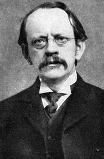
Fig. 1.4
JJ Thomson
Thomson’s investigations led eventually to the definitive proof of the particulate nature of cathode rays.11 Prior experiments of attempting to deflect the cathode rays by an electrostatic field were imprecise due to the imperfect vacuum of the tubes manufactured for these experiments. Such imperfections meant that the positive ions which had been created by cathode rays colliding with remnant gas atoms within the tube would be attracted to the cathode and create a shielding electric field of charge to reduce the net intensity of the field. But Thomson had created tubes with exquisitely high vacuums so that this field-masking problem did not occur and he could measure accurately the electric deflection of the cathode ray. The combination of electrostatic magnetic fields allowed the measurement of the electron velocity,  , through
  where e is the electric charge of the electron, E is the electric field and B is the magnetic field (Thomson 1897). The velocity was found to be of the order of 1.5 × 10⁷ m s−1 which, again, implied that the cathode ray mass was likely to be much less than that of an atom. Thomson determined the ratio of the cathode ray mass to charge through two particularly elegant experiments. In the first, he bombarded a target with a known thermal capacity, C, with a beam of cathode rays over a fixed period of time. The total charge carried by the beam is

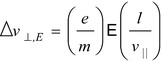
where N is the number of the particles making up the cathode ray beam during the time of irradiation and e is the electric charge carried by each. For an anode that is much thicker than the range of the cathode rays, all of the kinetic energy of this bolus of cathode rays will be absorbed by the target. The temperature of the target will, as a result, be raised by an amount ΔT determined through
where m is the mass of the individual cathode ray particle and v || is the velocity (the need for the || subscript to identify that the velocity is parallel to the cathode–anode axis will become soon apparent). As the cathode ray was known to be charged and deflected in a magnetic field B, the product of its radius of curvature in the field and B is given by
, through where e is the electric charge of the electron, E is the electric field and B is the magnetic field (Thomson 1897). The velocity was found to be of the order of 1.5 × 10⁷ m s−1 which, again, implied that the cathode ray mass was likely to be much less than that of an atom. Thomson determined the ratio of the cathode ray mass to charge through two particularly elegant experiments. In the first, he bombarded a target with a known thermal capacity, C, with a beam of cathode rays over a fixed period of time. The total charge carried by the beam is(1.1)
(1.2)
(1.3)
This quantity, the particle momentum per unit charge, is also known as the magnetic rigidity. From these equations, the mass-to-charge ratio of the elementary particle making up the cathode ray is given in terms of measurable quantities:
(1.4)
Thomson’s second experiment used coterminous electrostatic and magnetic fields. Consider the cathode ray (particle) of velocity v || traversing a length l across which an electric field  orthogonal to the direction of travel exists. The time that the particle spends within the field is
  during which it will experience a force e
  perpendicular to the direction of travel. As the force is constant over this distance, the net change in velocity normal to the direction of travel is
orthogonal to the direction of travel exists. The time that the particle spends within the field is during which it will experience a force e perpendicular to the direction of travel. As the force is constant over this distance, the net change in velocity normal to the direction of travel is(1.5)
The angle of deflection caused by this electric field is

(1.6)
A magnetic field B was then introduced and directed along the axis mutually perpendicular to both the electric field and the cathode–anode axis. The net change in the velocity orthogonal to the cathode ray’s direction (and antiparallel to that caused by the electron field) as a result of the magnetic field is
with an associated angle of deflection:
(1.7)
(1.8)


By adjusting the magnetic field B, Thomson was able to obtain the force-equalising condition of  (i.e. cancelling the deflection caused by the electric field) so that (1.9) yields

which also provides the mass-to-charge ratio in terms of measurable quantities. In both experiments, Thomson obtained a value for  equivalent to about 5.7 × 10⁻¹² kg/C for the cathode ray, a value which is some three orders of magnitude less than that of the 1.6 × 10⁻⁸ kg/C value that had been prior known as the smallest
  and which had been obtained for the hydrogen ion (proton) in electrolysis.
(i.e. cancelling the deflection caused by the electric field) so that (1.9) yields(1.10)
equivalent to about 5.7 × 10⁻¹² kg/C for the cathode ray, a value which is some three orders of magnitude less than that of the 1.6 × 10⁻⁸ kg/C value that had been prior known as the smallest and which had been obtained for the hydrogen ion (proton) in electrolysis.Finally, some 38 years after its discovery, Thomson was able to present the fact that the cathode ray was a particulate, with a negative electric charge and a mass of about 1/2,000th that of the hydrogen atom. He labelled this particulate a ‘negative corpuscle’, but this was subsequently renamed as the ‘electron’, a name coined earlier in 1894 by George Stoney as the fundamental unit of electric charge. The first subatomic particle and its basic characteristics of mass and electric charge had been identified and characterised. The electron, and its rate of energy loss as it moves through matter, will be very much a focus of this book. But we shall now look at the creation of other moving charged particles of relevance to medicine.
1.2.5 α- and β-Particles
Radioactivity is shown to be accompanied by chemical changes in which new types of matter are being continually produced – The conclusion is drawn that these chemical changes must be sub-atomic in character.
—Ernest Rutherford
Although the α- and β-particles are two entirely different physical entities, a doubly ionised helium atom and an electron (or positron), respectively, their coincident discoveries and investigations require that they be examined in parallel.12
Whereas the electron was the first subatomic particle to have been discovered, the manner of its production was artificial in that it required the thermionic emission of electrons from a cathode and their acceleration within an evacuated tube towards an anode. On the other hand, natural radioactivity, discovered serendipitously by Henri Becquerel in 1896 by noting the effects of the emissions of a uranium salt on photographic emulsion (Becquerel 1896), is a natural source of subatomic particles which has played and continues to play significant roles in medical radiation physics. Radioactive decay of nuclei leads, in the main, to the production of α- and β-particles. The medical application of the decelerated α-particle resulting from radioactive decay, which is the 4He nucleus, is exclusively therapeutic due to its short range in tissue. Over its short range, it deposits its kinetic energy tissue within a small volume consisting typically of only a few cells and yields a high and localised absorbed dose. As the short range of the α-particle does not enable it to exit tissue and be detected externally in order to form a diagnostic image, its use is relegated to the treatment of malignant disease in radionuclide therapy, as will be discussed.
On the other hand, the β-particle, which is either an electron or a positron that is emitted through nuclear decay, has both diagnostic and therapeutic applications in medicine. In its modern application, the positively charged β-particle, the positron, can annihilate with a nearby electron, resulting in the production of a pair of collinear γ-rays each with an energy equal to the rest masses of the electron and positron and which can be detected externally in order to form a diagnostic image in what is referred to as positron emission tomography (PET). On the other hand, the negatively charged β-particle, the electron, decelerates and produces an absorbed dose. The electron will tend to have a greater range than α-particles and, hence, the associated absorbed dose spatial distribution will be less localised. However, unlike the α-particle in traversing a medium, the electron can also undergo radiative loss through the production of bremsstrahlung which, in special circumstances, can be imaged in soft tissue, although this is rarely performed in nuclear medicine clinical practice.
The discovery of, and the assignation of the nomenclature to, α– and β-radiation from radioactive decay is attributed to Ernest Rutherford (Fig. 1.5), although he had initially misunderstood the physical nature of both.
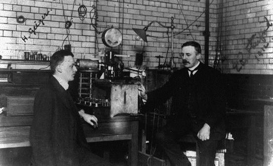
Fig. 1.5
Ernest Rutherford (right) and Hans Geiger (left) (Courtesy and © of Alexander Turnbull Library, Wellington, New Zealand)
The discoveries of these two radiations evolved out of his experimental work through which he measured the differential penetrations through aluminium foils of the emitted radiations resulting from the nuclear decay of uranium. Even though the partitioning of the emitted radiation into two components was Rutherford’s discovery, Becquerel had earlier observed that the radiation emitted by the uranium salt appeared to consist of components which had differential absorption properties.
A significant feature of this experimental work leading to the discovery of the α- and β-radiations was the nature of the radiation detector used by Rutherford. Prior work in the nascent field of radioactivity research had been dominated by the use of the photographic emulsion as a detector. Emulsion consists of silver bromide grains suspended in a gelatine matrix which are sensitised when radiation deposits energy in them through ionisation. These grains remain in this sensitised state, thus storing a latent image of the ionisation spatial pattern. During the development process, these sensitised grains are converted to metallic silver which affects surrounding silver molecules and increases the visibility of an ionisation, affecting a single silver bromide grain. Rutherford, however, considered emulsion as a slow and inefficient means of detecting radiation. In order to achieve the radiation detection sensitivity he required, Rutherford instead opted for gaseous ionisation detectors following his and Thomson’s earlier studies of the ionisation of gases exposed to x-rays (Thomson and Rutherford 1896; Rutherford 1897). Such observed ionisation was the product of photoelectric absorption and Compton scattering of photons by air molecules which resulted in the production of electrons and ions. The basic structure of the experiment performed by Rutherford in identifying α- and β-particles is shown in Fig. 1.6. This detector was an air ionisation chamber operated in the saturation mode as shown by the voltage–current curve in that figure. At low bias voltages, the electrons and positive ions that are produced following ionisation of the air molecules by the radiation have low drift velocities which result in a high probability of remaining within physical proximity and recombining, leading to a low ionisation current, I C. With an increasing bias voltage, the electrostatic field becomes sufficient to separate the electrons and positive ions prior to recombination. The current I C thus increases with bias voltage to reach a plateau (the ‘saturation mode’) reflecting the condition for which all of the ionisation products are collected.
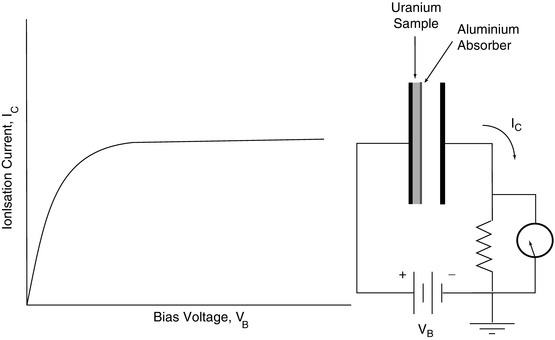
Fig. 1.6
Conceptual diagram of the ionisation detection apparatus used by Rutherford to identify the α- and β-particle components of the radiation emitted by uranium. As the two components had different electric charges, their detections required that the bias voltage be reversed for each (Refer to text for details)
In Rutherford’s experiment, a thin layer of a uranium salt placed on one electrode provided the source of ionisation and aluminium absorbers of various thicknesses were placed over the uranium salt, and the changes in I C were then measured as a function of the absorber thickness. Rutherford used an exponential model of the variation of the ionisation current with absorber thickness,  , where t is the thickness of absorber, and analysed the variation of the absorption parameter μ as a function of t. Charged particle radiations were stopped when the collision energy losses exceeded the particle’s incident kinetic energy. He determined that uranium emitted two types of radiations of different penetrability which he referred to as α and β in increasing order of penetration of the aluminium foil (Rutherford 1899). Despite what is commonly thought, Rutherford did not realise these to be the charged particles we now know them to be but, instead, considered them to be x-rays of two different energies. The differential penetration of the two particles in the foil is an immediate reflection of the collision stopping power, which is proportional to the square of the particle’s charge and the reciprocal of its mass.
, where t is the thickness of absorber, and analysed the variation of the absorption parameter μ as a function of t. Charged particle radiations were stopped when the collision energy losses exceeded the particle’s incident kinetic energy. He determined that uranium emitted two types of radiations of different penetrability which he referred to as α and β in increasing order of penetration of the aluminium foil (Rutherford 1899). Despite what is commonly thought, Rutherford did not realise these to be the charged particles we now know them to be but, instead, considered them to be x-rays of two different energies. The differential penetration of the two particles in the foil is an immediate reflection of the collision stopping power, which is proportional to the square of the particle’s charge and the reciprocal of its mass.Rutherford’s hypothesis of α- and β-radiations being photons of different energies began to succumb through the analysis using a magnetic field by Pierre Curie. The curvature of the trajectories of the β-radiations in the magnetic field demonstrated that this entity had an electric charge and, hence, was not a photon. Moreover, the direction of the trajectory revealed that it had a negative electric charge, and subsequent measurements of the mass to charge,  , proved unequivocally that the β-radiation was made up of fast electrons.13 On the other hand, the α-radiation could not be detected as deflecting in the magnetic field. This was the result of a combination of a weak magnetic field generated by the apparatus and the heavy mass of the α-particle. As the orbital radius of a particle with mass m, charge q and velocity v in a magnetic field B is
  , this combination of low magnetic field strength and high particle mass led to high values of r and the resulting imperceptible curvatures. Thus, further experimental investigation was required in order to identify the nature of the α-radiation.
, proved unequivocally that the β-radiation was made up of fast electrons.13 On the other hand, the α-radiation could not be detected as deflecting in the magnetic field. This was the result of a combination of a weak magnetic field generated by the apparatus and the heavy mass of the α-particle. As the orbital radius of a particle with mass m, charge q and velocity v in a magnetic field B is , this combination of low magnetic field strength and high particle mass led to high values of r and the resulting imperceptible curvatures. Thus, further experimental investigation was required in order to identify the nature of the α-radiation.It was the Curies who continued the investigation by using intense radioactive sources of radium and polonium which produced copious fluxes of α-particles. Of particular interest to our subject of charged particle energy loss, Pierre Curie measured a finite range of 6.7 cm in air for the α-radiation emitted by radium salts. Beyond that distance, the α-radiation failed to produce any ionisation in the detector. He found that this range was independent of the activity of the radium or of its chemical properties (Curie 1900a). We now know that this finite range is a function of the kinetic energy of the α-radiation and the properties of the absorbing material (in this case, air). The activity and chemical composition of the source of α-particles could in no way bear any influence on the result. Independently, Marie Curie measured the relative differential loss in ionisation of the α-radiation,  , and found that this ratio of ionisation loss increased with penetration distance (Curie 1900b). Unknowingly, she had discovered that the collision stopping power is inversely proportional to the square of the particle’s velocity – that is, the slower a particle moves through a medium due to previous energy transfers to the medium, the more rapidly it loses kinetic energy. While at the Adelaide University, William H Bragg (Bragg and Kleeman 1905) continued this work and showed that this energy deposition increased momentously near the end of the α-particle’s range. This feature is referred to as the Bragg peak and is one of the important elements of hadron therapy, as to be discussed.
, and found that this ratio of ionisation loss increased with penetration distance (Curie 1900b). Unknowingly, she had discovered that the collision stopping power is inversely proportional to the square of the particle’s velocity – that is, the slower a particle moves through a medium due to previous energy transfers to the medium, the more rapidly it loses kinetic energy. While at the Adelaide University, William H Bragg (Bragg and Kleeman 1905) continued this work and showed that this energy deposition increased momentously near the end of the α-particle’s range. This feature is referred to as the Bragg peak and is one of the important elements of hadron therapy, as to be discussed.In a further series of experiments, Becquerel was able to demonstrate that the α-radiation was not readily scattered in air and made diffuse. Using polonium as a source of α-radiation, he was able to image the sharp shadow of a wire on a photographic plate. We now recognise this inability to detect scattering in air as a consequence of the combination of the α-particle’s heavy mass and the low physical density of air.
However, Rutherford was able to demonstrate that α-particles could be scattered by materials and, in so doing, determined the large electric fields involved by using the experimental arrangement of Fig. 1.7.
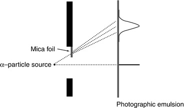
Fig. 1.7
Conceptualisation of the Rutherford experiment demonstrating that α-particles are scattered and spatially distributed by matter and the evaluation of the electric field strength required to achieve this (See text for details)
A sharply defined source of α-radiation was created using a wire coated with radium and a photographic emulsion was used as the detector. The α-particles were allowed to pass through a slit in a collimator and impinge on the emulsion. A thin sheet of mica with a thickness equivalent to that of 3.5 cm of air covered part of the slit. α-particles passing through the air and the foil would undergo scattering as a consequence of Coulomb interactions with the atoms and which would result in the deflection of the α-particles from their original trajectories. As to be derived in Chap. 4, the probability of Coulomb scatter through the angle θ is proportional to  . Hence, the scattering will be predominantly forward directed. Along the extended pathway of air, the α-particles will undergo multiple scatter with a net zero scattering angle integrated over the entire path length at the position of the detector. Those that pass through the mica foil will also be scattered but, due to the lever-arm effect and the mean zero scattering through air as shown in Fig. 1.7, will demonstrate an angular deviation at the position of the emulsion. By following the same route of development of (1.6), it can be readily shown that the electric field within the atoms of the mica to cause such a deflection is given by the expression

where E 0 is the kinetic energy of the α-particle, θ is the mean angle of scattering, e is the fundamental unit of electric charge and l is the linear thickness of the electric foil. An order-of-magnitude estimate of the strength of this electric field is obtained readily from (1.11). For example, the α-particle’s kinetic energy will be of the order of 5 MeV and the measured mean scattering angle was reported to be 2° or 35 mrad. The air-equivalent thickness of the mica yields an areal density of about 4.2 mg/cm2 which, for a density of 3 g/cm3 for mica, yields a thickness of 14 μm for the mica foil. Using these values in (1.11) yields an electric field E value of 1.25 × 10⁸ V/cm, thus demonstrating how a simple experiment can yield the magnitude of the Coulomb interaction causing the scatter and which will dominate the discussions of this book.
. Hence, the scattering will be predominantly forward directed. Along the extended pathway of air, the α-particles will undergo multiple scatter with a net zero scattering angle integrated over the entire path length at the position of the detector. Those that pass through the mica foil will also be scattered but, due to the lever-arm effect and the mean zero scattering through air as shown in Fig. 1.7, will demonstrate an angular deviation at the position of the emulsion. By following the same route of development of (1.6), it can be readily shown that the electric field within the atoms of the mica to cause such a deflection is given by the expression(1.11)
Rutherford had earlier resumed his examination of the problem of identifying the nature of the α-particle with the use of an intense magnetic field and a particularly intense radium source that had been provided him by the Curies. He demonstrated that the α-radiation was made up of positively charged particles and led to the suggestion, from the charge-to-mass ratio, that the α-particle could be the 4He nucleus (Rutherford 1903). This proof arose from the experimental results of Rutherford and Royds (1909). By collecting the α-particles from a glass tube containing radon gas that had traversed the extremely thin wall of the tube (and collected electrons from the glass in the process to be neutralised), compressing the resultant gas, and then by observing the optical spectrum resulting from an electric discharge through the captured gas, they demonstrated that the collected gas was helium. In conclusion, the α-particle was a cluster composed of, as we now know, two neutrons and two protons.
Experimental investigations of the rates at which α- and β-particles lost velocity while traversing material began in earnest at around this time at the Cavendish Laboratory in Cambridge and at Manchester. This work can probably be considered to have begun with Rutherford in 1906 using α-particles, with further refinements by Darwin and Geiger. The latter had determined that the α-particle velocity v as it traverses air could be described by the empirical relationship  , where v 0 is the original velocity, t is the thickness of air and b is a constant of proportionality. Experimental study of the β-particle proved to be more difficult than those of the α-particle. This difficulty was a consequence of the greater amount of scatter due to the β-particle’s much lower mass, the confounding effects of characteristic x-ray production caused by atomic relaxation resulting from its ionisation of the medium, bremsstrahlung, and the fact that the β-particles exhibited a velocity spectrum due to what we now know as the consequence of the three-body final state of nuclear β-decay,
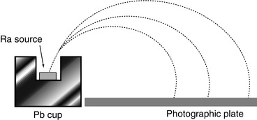
  . But even at this early time, elegant experiments were capable of extracting much detail of this phenomenon. Strutt’s measurements of the assumed exponential absorption of β-particles failed to find an absorption parameter μ that was independent of absorber thickness (Strutt 1900). This suggested a heterogeneity in the energies of the β-particles emitted from β-decay. Perhaps one of the simplest, yet most powerful, experiments to demonstrate the fact that the β-particles had a momentum spectrum was that of Becquerel as shown in Fig. 1.8. A radium source was placed within a lead cup and a magnetic field applied. The β-particles emitted during the radium’s decay were then bent into orbits impinging on a photographic plate so that the physical spread of the darkening of the film was reflective of the spread of β-particle velocities (Becquerel 1903).
, where v 0 is the original velocity, t is the thickness of air and b is a constant of proportionality. Experimental study of the β-particle proved to be more difficult than those of the α-particle. This difficulty was a consequence of the greater amount of scatter due to the β-particle’s much lower mass, the confounding effects of characteristic x-ray production caused by atomic relaxation resulting from its ionisation of the medium, bremsstrahlung, and the fact that the β-particles exhibited a velocity spectrum due to what we now know as the consequence of the three-body final state of nuclear β-decay, . But even at this early time, elegant experiments were capable of extracting much detail of this phenomenon. Strutt’s measurements of the assumed exponential absorption of β-particles failed to find an absorption parameter μ that was independent of absorber thickness (Strutt 1900). This suggested a heterogeneity in the energies of the β-particles emitted from β-decay. Perhaps one of the simplest, yet most powerful, experiments to demonstrate the fact that the β-particles had a momentum spectrum was that of Becquerel as shown in Fig. 1.8. A radium source was placed within a lead cup and a magnetic field applied. The β-particles emitted during the radium’s decay were then bent into orbits impinging on a photographic plate so that the physical spread of the darkening of the film was reflective of the spread of β-particle velocities (Becquerel 1903).Fig. 1.8
Experiment used by Becquerel to study the spectrum of β-particle velocities
1.2.6 Internal Conversion and Coster–Krönig Electrons
Nuclear β-decay is not the only means by which electrons are emitted in a radioactive process. Non-radiative transitions and atomic relaxation processes can also result in the production of moving electrons. Unlike β-particles, these electrons are monoenergetic, while internal conversion electrons can have energies and ranges comparable to those typical of nuclear β-decay; Auger and Coster–Krönig electrons have, in general, much reduced energies and ranges.
Internal conversion (IC) is a non-radiative decay process which may be made available to an excited nucleus. As low-orbital (K and, to a lesser degree, L) electrons have wavefunctions that can overlap that of the nucleus, it is possible for the nucleus to transfer energy to the electron directly without the presence of an intermediate γ-ray, but through a virtual photon. In other words, IC is not a photoelectric absorption event in which a γ-ray is emitted by the de-exciting nucleus and absorbed by an atomic electron.14 The electron is subsequently ejected with energy equal to the difference between the nuclear excitation energy and the atomic electron’s binding energy. The IC electron plays a significant role in internal radiation dosimetry calculation (Smith et al. 1965).
A key consequence of the ejection of an IC electron is that of a hole in the orbital from which the electron was removed. This will result in the transition of an electron from a higher orbital to fill this hole (Fig. 1.9). The transition can be radiative with the emission of a characteristic x-ray with an energy equal to the difference between the two orbital binding energies. However, this energy can also be directed towards another electron which is then ejected to create another hole. Another transition can occur to fill this new hole and the difference in energy between the two orbitals transferred to yet another electron which is ejected, etc. This process is known as the Auger cascade and results in the ejection of multiple low-energy electrons. Auger electrons were discovered and explained by Lise Meitner in 1923, but only in the course of a longer treatise on the β-decay spectrum of 234Th which, as a result, this discovery received limited attention. Two years later, Pierre Auger discovered these eponymous electrons independently by observing their tracks in a Wilson cloud chamber.15
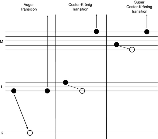
Fig. 1.9
Non-radiative Auger and Coster–Krönig transitions
If the electron vacancy is in a different orbital, the process is referred to as an Auger transition. Coster–Krönig and super Coster–Krönig transitions occur within suborbital levels. A Coster–Krönig transition is one in which the transiting electron and vacancy are in the same main orbit, but the ejected electron is from a different main orbit. A super Coster–Krönig transition is one in which the transiting electron, vacancy and ejected electron are all from the same main orbit.16
The absorbed doses associated with Auger transitions can be significant and, if in the vicinity of a radiosensitive biological target, lead to significant biological effects (Boswell and Brechbiel 2005). Auger electrons will tend to have low kinetic energies and, subsequently, low ranges of penetration into tissue. Should an Auger electron-emitting radionuclide be brought into close proximity of the radiosensitive centre of a cell (the nucleus), significant damage leading to cell death can occur. This could be a desirable effect for therapy but could also be of radiation protection concern in diagnostic applications if the diagnostic radiopharmaceutical uses a radionuclide which is an Auger-electron emitter. Moreover, another result of an Auger cascade is that of a highly charged ion which, if in the vicinity of radiosensitive cell structures, can also cause biological damage. Hence, the roles played by Auger electrons in therapeutic nuclear medicine and in the radiation protection considerations of diagnostic nuclear medicine are of considerable interest due to their low energy and the  dependence of the collision energy loss. Table 1.2 summarises the Auger-electron emission characteristics of a number of radionuclides used in nuclear medicine.
dependence of the collision energy loss. Table 1.2 summarises the Auger-electron emission characteristics of a number of radionuclides used in nuclear medicine.Table 1.2
Total Auger-electron yield for radionuclides commonly used in nuclear medicine
Radionuclide | Mean yield of Auger electrons per decay |
|---|---|
67Ga | 4.7 |
99mTc | 4.0 |
111In | 14.7 |
123I | 14.9 |
201Tl | 36.9 |
1.2.7 Protons
The proton is the lightest baryon and its existence had been inferred as early as 1808 through Dalton’s gravimetric weight measurements which had implied that the elements were made up of integral constituents. This was followed by Proust’s hypothesis in 1815 that all elements were integral multiples of the hydrogen atom, which he had termed as the protyle. The proton had been recognised as being a hydrogen ion through, for example, electrolysis. It was inferred as a nuclear constituent gravimetrically and, to some degree, by Rutherford’s interpretation of the results of Geiger’s and Marsden’s experiment of scattering α-particles from gold foils. The definitive proof of the existence of the proton as a subnuclear particle can be traced to Rutherford’s investigations of the scintillations observed on a zinc sulphide screen at one end of a glass tube and a radium source of α-particles at the other. The tube could be filled with a variety of gases. Critically, the scintillation screen was placed at a distance from the radium source beyond the α-particle range, and a transverse magnetic field was applied to deflect β-particles emitted by the radium decay from reaching the screen (Rutherford 1919). As a consequence, any scintillations observed would be due to any new particles that had been created by interactions between the α-particles and the gas and which had a range greater than the α-particle and a magnetic rigidity exceeding that of a β-particle. When the tube was filled with either dry air or nitrogen, Rutherford observed scintillations which satisfied the criteria of the range and mass of the secondary particle sought. As the former is dependent on electric charge, this result indicated that these scintillations were due to a charged particle with a unit charge of e and a mass intermediate to that of an electron and that of a 4He++ ion, in other words, the proton. As the rate of scintillations occurring was 1.25 times greater for pure nitrogen than for air, it was deduced that these scintillations were caused by the interactions between the α-particles and the nitrogen nuclei. On the basis of this observation, Rutherford hypothesised that the nitrogen nucleus was composed of three helium nuclei and two hydrogen nuclei (recall that this experiment was performed before the discovery of the neutron by Chadwick). In this case, he conjectured that the α-particle collided with the nitrogen nucleus and imparted sufficient momentum to a valence proton to eject it from the nucleus.
Related posts:
Stay updated, free articles. Join our Telegram channel

Full access? Get Clinical Tree


