Fig. 1.
(left) Brain images of MS patients with (right) lesions segmented by experts. We show (a) a volume with heavy peri-ventricular lesion load, (b) volume with supra-ventricular lesions, and (c) volume with juxta-cortical lesions. The different shapes, sizes, positions and intensities make lesion segmentation challenging.
Although various automatic approaches have been developed for the segmentation of MS lesions, their adoption into real clinical practice has been limited. This is primarily due to strong simplifying assumptions, which restrict the robustness to variability displayed in large clinical datasets [2]. For example, techniques that define lesions as outliers of healthy class distributions [3, 7] risk missing a large set of subtle lesions located throughout the brain, for which these assumptions are violated. Techniques based on topological features and template matching (e.g. [10]) presume that lesion shape can easily be modelled by a set of candidate lesion shapes, which is difficult to achieve in practice. Finally, most techniques are tested on synthetic lesion data, or on the limited MICCAI Challenge dataset [4, 7], neither of which reflects the variability present in large clinical datasets.
Various MRF techniques have been proposed for pathology segmentation [3, 11] but typically only class relationships are reflected in the priors (e.g. Ising models). However, traditional MRFs tend to smooth class labels excessively, and hence may lead to the removal of smaller MS lesions. To alleviate this problem, a modified MRF [9] has been proposed, which models both voxel intensities and intensity differences in the cliques. However, a local model of a voxel and its neighbourhood is insufficient for this task, and a more global view of context is necessary for accurate classification. Recently, several different, multi-level graphical models have been introduced for segmentation of pathologies [12, 13]. However, none have been designed for the unique context of MS lesion segmentation.
In this work, we present IMaGe, a new, iterative, two-stage, probabilistic, graphical model for the detection and segmentation of MS lesions in multi-channel MRI. The goal of this architecture is to take advantage of both local information, as well as global context, in order to remove false assertions and refine boundaries. The lower level consists of nodes associated with each voxel, and models the intensities of healthy tissues and lesions, as in [9]. It produces a set of lesion candidates, passed to the higher level, whose goal is to determine which of these candidates are indeed lesions, by looking at a larger context around each region. The higher level consists of a non-lattice based MRF (whose structure is not a regular, uniform grid). Each node corresponds to a contiguous region of voxels currently labelled with the same class, and nodes are connected if the corresponding regions have at least one voxel adjacent to the other region. Each region is modelled using both intensity and textural features, and the relations between different regions are also considered. The class label computed based on this information, as well as the texture information, is then passed to the lower level. Inference alternates between the two levels, until a consensus is reached about the lesion candidates, or a given number of iterations has elapsed. Figure 2 illustrates this process.
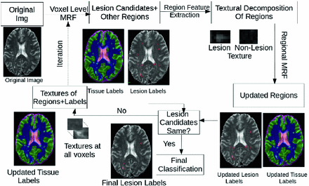
Fig. 2.
Flowchart of the proposed approach. The multimodal MRI are processed by a 2 stage iterative MRF. At the bottom level, a voxel based MRF identifies potential lesion voxels, as well as other tissue classes. Contiguous voxels of a particular tissue type are grouped into regions. A higher, non-lattice based MRF is then constructed, in which each node corresponds to a region, and edges are defined based on neighbourhood relationships between regions. Regional features such as textures are extracted from each region. The goal of this MRF is to evaluate the probability of candidate lesions, based on group intensity, texture, and neighbouring regions. If the resulting labels have changed at this stage, the labels and textures are then propogated back down to the voxel-level MRF. This process of iterative inference continues until convergence.
IMaGe is trained on 660 MS patient MRI volumes from a clinical trial involving 174 centres. In order to test the robustness of the framework to different trial data, testing was performed on a different clinical trial data set of 535 MRI MS patient volumes from 128 centres. Both datasets include T1, T2, PD and FLAIR contrasts. We compared IMaGe to a recent MRF technique based on FLAIR [5], a traditional MRF, and the result of the voxel-based MRF [9]. IMaGe outperformed the competitors based on sensitivity and Positive Predictive Value, particularly in the context of smaller lesion detection (i.e. in the 3–10 voxel range), comprising around 40 % of the clinical trial dataset. These small lesions often constitute a very small portion of the total volume of the lesions, but it is important to detect them in clinical settings since the activity of the disease is measured by the number of lesions, both large and small.
2 Methodology
Given a multichannel MRI volume, the task is to identify the voxels corresponding to MS lesions. The proposed hierarchical MRF technique identifies potential lesion candidates at the lower level, and the validity of the candidates is inferred at the higher level, where the lesion boundaries are also refined. We describe in detail the framework in Fig. 2.
2.1 Voxel-Level MRF
Traditional voxel level MRFs [8, 11] are typically lattice-based and infer the class of a voxel using observations local to that voxel (such as intensity) and the classes of the neighbouring voxels. However, this process tends to smooth over small patches of voxels whose class differs from their neighbours. This is problematic for MS lesions, which tend to be very small (3–10 voxels). To alleviate this problem, we employ a modified MRF at the voxel level, as in [9], which uses at each voxel the contrast of the local observation with those of the neighbours. Specifically, at each node we consider the observation to include the intensity difference between the corresponding voxel and its neighbours.
The MRF is structured as a regular lattice, with a node for each voxel and connectivity as depicted in Fig. 3. Let Q be the number of voxels in the volume, and  denote the vector of multimodal intensities at voxel i and
  denote i’s neighbourhood (Fig. 3). The goal is to infer the class label
  , corresponding to voxel i’s tissue type (lesion, white matter (WM), grey matter (GM), cerebro-spinal fluid (CSF) or partial volume1 (PV)). Let
  denote the vector of intensities of the voxels in
  and
and  denote the vector of class labels for these voxels. Let
  be the collection of all class labels for the corresponding voxels in the volume, and
  be the corresponding intensities. The goal is to compute
  , which in an MRF is given by:
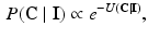
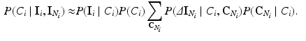
where  is the energy of the configuration. Following [9], the posterior probability of class
  is given by:
where the sums marginalize over all combinations of class labels that can be assigned to the neighbourhood voxels. In Eq. (2),  is the prior probability at voxel i,
  represents the probability of class transitions in the neighbourhood,
  is the likelihood of
  given class
  and
and 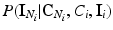 models the likelihood of the intensity of the neighbouring voxels, given their classes and the information at voxel i.
denote the vector of multimodal intensities at voxel i and denote i’s neighbourhood (Fig. 3). The goal is to infer the class label , corresponding to voxel i’s tissue type (lesion, white matter (WM), grey matter (GM), cerebro-spinal fluid (CSF) or partial volume1 (PV)). Let denote the vector of intensities of the voxels in and denote the vector of class labels for these voxels. Let be the collection of all class labels for the corresponding voxels in the volume, and be the corresponding intensities. The goal is to compute , which in an MRF is given by:(1)
is the energy of the configuration. Following [9], the posterior probability of class is given by:(2)
is the prior probability at voxel i, represents the probability of class transitions in the neighbourhood, is the likelihood of given class and models the likelihood of the intensity of the neighbouring voxels, given their classes and the information at voxel i.Fig. 3.
(a) The regular MRF model and (b) the MRF model used in [9]. Note that the neighbouring intensities are considered in the computation of the label at every node i in this model.
Let  be defined as the intensity difference between
  and
and  in the clique (see Sect. 3.1 for details on computing intensity differences). Since
  can be computed deterministically from
  and
and  , in Eq. 2, we replace
  with
with 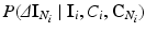 . We can also assume that the difference in intensity between a voxel and its neighbours depends on the classes in the neighbourhood, but not on the absolute intensity of the voxel itself, and hence we can replace
 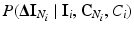 with
with 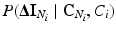 . Furthermore, we assume that the intensity of a voxel is conditionally independent of the neighbourhood classes, given the class label at the voxel. Hence, we can replace
  with
with  . With these assumptions, Eq. (2) simplifies to:
Using Eqs. 1 and 3, the Gibbs energy function is given by: 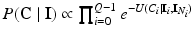 . To infer the class labels, the total energy must be minimised. The energy at each voxel i can be expressed as:
where k indexes over all the possible cliques in  and j indexes over all the possible elements of clique k,
  is the potential associated with the relationship between
  and the vector of classes in the jth clique,
  , and
, and  is a weighting parameter used to handle the differences between inter-slice and intra-slice distances.
be defined as the intensity difference between and in the clique (see Sect. 3.1 for details on computing intensity differences). Since can be computed deterministically from and , in Eq. 2, we replace with . We can also assume that the difference in intensity between a voxel and its neighbours depends on the classes in the neighbourhood, but not on the absolute intensity of the voxel itself, and hence we can replace with . Furthermore, we assume that the intensity of a voxel is conditionally independent of the neighbourhood classes, given the class label at the voxel. Hence, we can replace with . With these assumptions, Eq. (2) simplifies to:(3)
. To infer the class labels, the total energy must be minimised. The energy at each voxel i can be expressed as:(4)
and j indexes over all the possible elements of clique k, is the potential associated with the relationship between and the vector of classes in the jth clique, , and is a weighting parameter used to handle the differences between inter-slice and intra-slice distances.Related posts:
 Stable Overlapping Replicator Dynamics for Multimodal Brain Subnetwork Identification
 PET Reconstruction with Sparse Image Representation and Anatomical Priors
 Method to Discover Genetically Driven Image Biomarkers
Stay updated, free articles. Join our Telegram channel

Full access? Get Clinical Tree


