Joint Acquisition-Estimation Framework for MR Phase Imaging

could be written as:

$\begin{aligned} \mathbf{m}_{k,c} (x,y) = \rho _{k,c}(x,y)\exp \big \{i(\phi _{0,c}(x,y)+2\pi \varDelta B(x,y) \text {TE}_k )\big \} + \mathbf{w}(x,y) \end{aligned}$

(1)

where $\rho _{k,c}(x,y)$ is the decayed magnitude at echo time TE

modulated by the sensitivity of channel c, $2\pi \varDelta B(x,y) \text {TE}_k$ is the underlying tissue phase value and $\phi _{0,c}(x,y)$ is the channel-dependent phase offset of channel c. $\phi _{0,c}(x,y)$ varies spatially due to factors such as the distance between the excited spins and the coil, the length of the coil’s cables, and electronic delay [9]. Strictly speaking, $\phi _{0,c}(x,y)$ also varies with time due to drifts in frequency synthesizer and/or imperfections in the centering of k-space [5]. The term $\varDelta B(x,y)$ accounts for all deviations from the main magnetic field at location (x, y) which are due to both, inherent local tissue properties (which induce such local changes), as well as global object coil-loading effects. We refer here to $\varDelta B(x,y)$ as “tissue frequency.” Finally, the noise term $\mathbf{w}(x,y)$ in each voxel is drawn i.i.d. from a complex Gaussian Random Variable (RV), i.e. $\mathbf{w} = \mathbf{w}_R + i \mathbf{w}_I$ , $\mathbf{w}_R,\mathbf{w}_I\!\sim \!\mathcal {N}(0,\sigma _w)$ . Quantitation from MR phase requires the extraction of the term $\varDelta B(x,y)$ from the measurements $\mathbf{m}_{k,c}(x,y)$ . However, instead of the absolute phase, we are restricted to measuring the numerically computed angle of $\mathbf{m}_{k,c}(x,y)$ , namely,

$\begin{aligned} \varvec{\Psi }_{k,c} (x,y) = \phi _{0,c} (x,y) + 2\pi \varDelta B (x,y) \text {TE}_k + \varvec{\Omega }_{k,c} (x,y) + 2\pi \mathbf{r}_{k,c} (x,y), \end{aligned}$

(2)

where $\varvec{\Omega }_{k,c} (x,y)$ is the phase contribution of the additive noise term and $\mathbf{r}_{k,c} (x,y)$ is a phase wrapping integer which forces the sum of the first three terms on the right side of (2) to be in the range $[-\pi ,\pi )$ . Note that, because the noise’s contribution in the phase depends on $\rho _{k,c}(x,y)$ , both $\varvec{\Omega }_{k,c}(x,y)$ and $\mathbf{r}_{k,c} (x,y)$ are a function of $\text {TE}_k$ and channel c. It is clear from (2) that there are four unknowns in the angle measurements $\varvec{\Psi }_{k,c} (x,y)$ : the parameter of interest $\varDelta B(x,y)$ , and 3 additional sources of ambiguity (phase offset, noise and phase-wrapping integer).

Phase Offsets $\varvec{\phi }_\mathbf{0,c}$ : Existing methods attempt to address this challenge by either (a) referencing $\mathbf{m}_{k,c}$ to a known coil or given location (equalization) [4, 7], (b) estimating then eliminating $\phi _{0,c}$ [6, 8] or (c) inverting the sensitivity profile of the coil-array [10, 12]. Equalization methods are sensitive to coil geometry, often resulting in severe artifacts in areas of low SNR, or areas of $\varDelta B$ variations. Cancelation methods suffer from an inherent SNR penalty, and require separate “reference” scans which assume that $\phi _{0,c}$ are temporally invariant [5]. Finally, inversion methods suffer from substantial errors/artifacts in areas of noise/poor regularization.

Phase Noise and Wrapping: The authors in [1] have shown that imaging the MR phase signal inherently trades off two types of errors: noise and phase wrapping. There, the authors have identified three phase imaging regimes: (I) a regime dominated by phase-wrapping, with reduced levels of noise, (II) a regime dominated by noise, with no phase-wrapping and (III) a regime where the phase signal needs to be disambiguated from both phase-wrapping and noise contributions. Most phase imaging methods operate in Regime III [1] where post-processing is relied on in order to perform phase unwrapping and denoising. As carefully documented in [9], phase unwrapping methods are not robust and often require expert-user intervention. Other methods proposed in [2] use a combination of short (Regime II) and long (Regime I) echo times in order to recover the phase signal using an ML framework. However, as shown in [1], such methods are suboptimal because (a) long echo acquisitions rely on short echo acquisitions (which induces error propagation) and (b) the phase is computed using echo referencing (which induces noise amplification). Furthermore, the method in [2] relies on spatial regularization which biases the estimate.

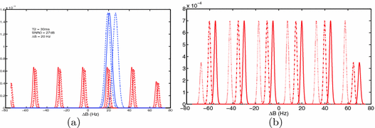
Fig. 1.

(a) Example likelihood functions, with $\phi _{0,c}=0$ , in a voxel where $\varDelta B$ = 20 Hz, SNR0=22 (27 dB) and T2*=30 ms. The family of blue lines correspond to $\mathcal {L}_{k,c}{(\varDelta B)}$ for different $\psi _{k,c}$ realizations, at TE = 5 ms. The red lines are $\mathcal {L}_{k,c}{(\varDelta B)}$ obtained at TE = 40 ms. (b) $\mathcal {L}_{k,c}{(\varDelta B)}$ for the same voxel as (a), at TE=40 ms, but obtained through 3 channels each with different phase offsets.

2 MAGPI: A Maximum-Likelihood Framework

2.1 Problem Formulation

The task here is to estimate $\varDelta B$ from $\varvec{\Psi }_{k,c}$ . The ML estimator is popular due to its optimality properties such as efficiency, sufficiency, consistency and invariance. We can show that the likelihood function for our problem, $\mathcal {L}_{k,c}$ , is given by:

$\begin{aligned} \mathcal {L}_{k,c}{(\varDelta B)} \triangleq \text {pr}\left( \varvec{\Psi }_{k,c} \!=\! \psi _{k,c} \big / \varDelta B\right) = \text {pr}\left( \varvec{\Omega }_{k,c} + 2\pi \mathbf{r}_{k,c}\!=\! \psi _{k,c}\! -\! 2\pi \varDelta B \text {TE}_k \!-\! \phi _{0,c} \right) \end{aligned}$

(3)

where $\psi _{k,c}$ is a realization of the random variable (RV) $\varvec{\Psi }_{k,c}$ . Note that, because the phase wrapping integer $\mathbf{r}_{k,c}$ depends on the phase noise RV $\varvec{\Omega }_{k,c}$ , this implies that $\mathbf{r}_{k,c}$ is also a (discrete) RV. Using the total probability theorem, and carrying on derivations not shown here, we can write:

$\begin{aligned} \mathcal {L}_{k,c}{(\varDelta B)} = \sum _r P(\mathbf{r}_{k,c}=r) {f}_{\varvec{\Omega }_{k,c}}\!(\psi _{k,c} - 2\pi \varDelta B \text {TE}_k - 2\pi r - \phi _{0,c}) \end{aligned}$

(4)

where $P(\mathbf{r}_{k,c}=r)$ is the probability of obtaining a given wrapping integer r and ${f}_{\varvec{\Omega }_{k,c}}$ is the PDF of the noise in channel c, at echo time k, each given by:

$\begin{aligned} \scriptstyle P(\mathbf{r}=r) = \frac{\sigma _{k,c} \sqrt{2}}{4\zeta _\text {max}} \left[ \frac{e^{-b_2^2} - e^{-a_2^2}}{\sqrt{\pi }} - a_2 \text {erf}(a_2) + b_2 \text {erf}(b_2) - \frac{e^{-b_1^2} - e^{-a_1^2}}{\sqrt{\pi }} + a_1 \text {erf}(a_1) - b_1 \text {erf}(b_1)\right] \end{aligned}$

(5)

$\begin{aligned} \text {where} \quad \scriptstyle a_1 = \frac{\left( \frac{2r-1}{2\text {TE}_k}-\zeta _\text {max}\right) }{\sqrt{2}\sigma _{k,c}}; b_1 = \frac{\left( \frac{2r+1}{2\text {TE}_k}-\zeta _\text {max}\right) }{\sqrt{2}\sigma _{k,c}}; a_2 = \frac{\left( \frac{2r-1}{2\text {TE}_k}+\zeta _\text {max}\right) }{\sqrt{2}\sigma _{k,c}}; b_2 = \frac{\left( \frac{2r+1}{2\text {TE}_k}+\zeta _\text {max}\right) }{\sqrt{2}\sigma _{k,c}} \end{aligned}$

(6)

and $\zeta _\text {max}$ is the maximum value of

, and,

(7)

and $\text {snr}_{k,c}$ is the magnitude-domain SNR in channel c at TE $$_k$$

. Note that our phase signal model does not assume any specific magnitude-decay model. We validated these theoretical predictions using numerical simulations and observed a close match (not shown here). We focus here on the dependence of the likelihood functions on TE $$_k$$

, $\varDelta B$ , T2* and SNR $_{0,c}$ . We plot in Fig. 1(a) two families of likelihood functions obtained at two different values of TE $$_k$$

. We ignore the channel offsets ( $\phi _{0,c} = 0,\forall c$ ) in this figure. We note the following: First, depending on the choice of TE $$_k$$

, the likelihood functions exhibit either sharp but multiple maxima (wrapping-dominated regimes), or a broad unimodal peak (noise-dominated regimes). Therefore, the likelihood function captures the inherent trade-offs between noise and phase wrapping with respect to the choice of TE $$_k$$

. Second, we note that repeated measurements (dashed family of lines) yield randomly shifted $\mathcal {L}_{k,c}{(\varDelta B)}$ . Measurements at the larger TE $$_k$$

result in a family of likelihood functions that are more tightly centered around the true $\varDelta B$ , as compared to the shorter TE $$_k$$

. We include the effects of the unknown phase offset in Fig. 1(b), where we plot example $\mathcal {L}_{k,c}{(\varDelta B)}$ for different channels c. Note that likelihoods in the same voxel are shifted with respect to one another by an unknown amount, $\phi _{0,c}$ . This example illustrates that maximizing the likelihood is not trivial due to: (1) the function either having multiple maxima or one maximum whose location is sensitive to noise and (2) the unknown $\phi _{0,c}$ .

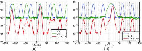
Fig. 2.

Example system likelihood functions obtained from individual dual-echo likelihoods. Note that the system likelihoods (red) are not subject to the same noise-phase wrapping trade offs as the dual-echo likelihoods (green and blue) (Color figure online).

2.2 Proposed Solution: MAGPI

Our proposed framework, coined MAGPI (Maximum AmbiGuity distance for Phase Imaging), acquires Multi-Echo Gradient Echo (MEGE) measurements from a collection of K echoes, and $$N_c$$

channels, within a single TR. The estimation step is described using the 3-pass process detailed below.

Pass I: Find the most likely $\varDelta B$ that explains the angle buildup between echoes. We can show that the angle buildup between any two echoes is:

$\begin{aligned} \varvec{\Delta \Psi }_{2:1,c} \triangleq \angle \left\{ \mathbf{m}_{2,c}\mathbf{m}_{1,c}^*\right\} = 2\pi \varDelta B \varDelta \text {TE}_{2:1} + \varvec{\Delta \Omega }_{2:1,c} + 2\pi \mathbf{r}_{2:1,c}, \end{aligned}$

(8)

where $\varDelta \text {TE}_{2:1} \triangleq \text {TE}_{2} - \text {TE}_{1}$ , $\varvec{\Delta \Omega }_{2:1,c} \triangleq \varvec{\Omega }_{2,c} - \varvec{\Omega }_{1,c}$ and $\mathbf{r}_{2:1,c}$ is a phase wrapping integer which forces the sum of the first two terms on the right side of (8) to be in the range $[-\pi ,\pi )$ . We note two differences in (8) as compared to (2). First, the relative phase buildup does not depend on $\phi _{0,c}$ . The second important difference is a reduced tissue phase amplification (due to multiplication with a smaller term, $\varDelta \text {TE}_{2:1}$ ) accompanied by noise amplification (two contributions from noise RVs). We will address this shortcoming in pass III below. The likelihood function, denoted by $\mathcal {L}_{2:1,c}{(\varDelta B)} \triangleq \text {pr}\!\left( \varvec{\Delta \Psi }_{2:1,c} \big / \varDelta B\right)$ , is now given by:

$\begin{aligned} \mathcal {L}_{2:1,c}{(\varDelta B)} = \! \sum _{r=-R}^{R} P(\mathbf{r}_{2:1,c}=r) {f}_{\varvec{\Delta \Omega }_{2:1,c}}\!(\varDelta \psi _{2:1,c} - 2\pi \varDelta B \varDelta \text {TE}_{2:1} - 2\pi r) \end{aligned}$