Fig. 3.1
System for applying shear waves to the abdomen for MR Elastography of the liver. All the add-on hardware elements are listed in the top row. Acoustic pressure waves (at 60 Hz) are generated by an active driver, located away from the magnetic field of the MRI unit, and transmitted via a flexible conductive tube to a passive driver placed over the anterior body wall. The left bottom diagram illustrates the location of the passive driver with respect to the liver in a coronal sketch. The right bottom diagram is an overview of the liver MRE examination setup
As illustrated in Fig. 3.1, patients are usually imaged in the supine position with the passive driver placed against the anterior body wall over the right lobe of the liver on the chest wall below the breast, held in place with an elastic band around the body. The placement of the passive driver can be standardized by using xiphisternum as the landmark for placing the center of the driver and mid clavicular line for placing over the right lobe of the liver. Continuous longitudinal vibrations at 60 Hz are generated by varying acoustic pressure waves transmitted from an active driver device via a PVC conductive tube.
Software (Pulse Sequence)
The measurement of motion with MR in medical applications has been motivated significantly by the desire for blood flow quantification and vascular system imaging [48]. In the 1990s, measurement of tissue mechanical properties using MR methods was demonstrated [9, 49]. MRE uses a modified phase-contrast imaging sequence to detect propagating shear waves within the tissue of interest. Depending on the specific application, the MRE sequence uses a conventional MR imaging sequence [e.g., GRE, spin echo (SE), balanced steady-state free precession (bSSFP), or echo planar imaging (EPI)] with the inclusion of additional motion-encoding gradients (MEGs), which allow shear waves with amplitudes in the micron range to be readily imaged [9, 49–55]. The MEGs are imposed along a specific direction and switched in polarity at an adjustable frequency. Trigger pulses synchronize the imaging sequence with the driving system to induce shear waves in the tissue, usually at the same frequency as the MEGs. In the received MR signal, a measurable phase shift caused by the cyclic motion of the spins in the presence of these MEGs can be used to calculate the displacement at each voxel, which provides a snapshot of the mechanical waves propagating within the tissue. By adjusting the phase offset between the mechanical excitation and the oscillating MEGs, wave images can be obtained for various time points of the vibration. Four phase offsets evenly spaced over 1 cycle of the motion are obtained in most experiments. This allows for the extraction of the harmonic component of the phase data at the driving frequency, giving the amplitude and the phase of the harmonic displacement at each point in space, which is the input to most MRE inversion algorithms.
A typical 2-D GRE MRE sequence (as shown in Fig. 3.2) has the following parameters (more in Table 3.1): 60 Hz continuous sinusoidal vibration, FOV = 30-42 cm, matrix = 256 × 64, flip angle = 30°, slice thickness = 10 mm, number of slices = 4, TR/TE = 50/20 ms, parallel imaging factor = 2, 4 evenly spaced phase offsets, and 1 pair of 60 Hz trapezoidal MEGs with zeroth and first moment nulling along the through-plane direction. Two spatial presaturation bands are applied on each side of the selected slice to reduce motion artifacts from blood flow. The total acquisition time is less than a minute, split into 4 breath holds.
Fig. 3.2
2D GRE MRE sequence. This sequence is a conventional gradient echo sequence with an additional motion-encoding gradient (MEG) applied along the slice selection direction to detect cyclic motion in the through-plane direction. Sequence provides options to select other motion-encoding directions. The MEG is designed to minimize zeroth and first gradient moments. The MEG and the acoustic driver are synchronized using trigger pulses provided by the imager. The phase offset (θ) between the two can be adjusted to acquire wave images at different phases of the cyclic motion
Table 3.1
Imaging parameters of a GRE–MRE sequence in liver MRE application
Parameters | Typical values |
|---|---|
Magnetic field strength | 1.5T |
Patient body habitus | Supine/feet first |
Orientation | Axial |
Field of view (FOV) | 30 ~ 42 cm (Patient-specific) |
Fractional phase FOV | 0.7–1.0 (Patient-specific) |
In-plane resolution | 256 × 64 |
Frequency direction | R/L |
TR/TE | 50/20 |
Slice thickness | 10 mm |
Number of slices | 4 |
Flip angle/number of echoes/ETL | 30/1/1 |
NEX/number of shots | 1/0 |
ASSET acceleration factor | 2 |
Active driver (resoundant system) frequency | 60 Hz |
Active driver (resoundant system) power | 50 % power |
MEG frequency/period | 60 Hz/16.7 ms |
Number of MEG gradient pairs | 1 |
MEG amplitude | 1.76 Gauss/cm (Machine dependent) |
MEG direction | slice direction |
Number of phase offsets | 4 |
Acquisition time | 54 s or less (four breath-hold) |
Several artifact reduction strategies are used to maintain high image quality. In order to obtain a consistent position of the liver and establish more reproducible breath-hold positions for each suspended respiration, subjects are asked to hold their breath at the end of expiration. Breath-hold technique scan time is shorter than would likely be achieved with a respiratory gated sequence [39]. In the application of MRE with passive drivers, bulk motion can induce signal loss, ghosting, and unwanted phase accumulation, as shown in the first row of Fig. 3.3. However, we want spins to accrue phase from applied sinusoidal motion only. In order to separate these two sources of phase accumulation, Gradient Moment Nulling (GMN) can be applied to the motion sensitizing gradient waveform. It is well known that so called 1-2-1 (pulse widths of the first and last lobe are half of the central lobe) gradient pulses inherently have their 0th and 1st moments nulled. By definition, moments are a linear operation. Therefore, multiple 1-2-1 pulses can be superimposed on each other to yield longer trains of GMN pulses. As shown in Fig. 3.2, one pair of bipolar motion sensitizing gradients with GMN had their 0th and 1st moments nulled without changing the sensitivity to the desired sinusoidal shear motions. Additionally, nulling the 1st moment of the motion sensitizing gradient waveform does not require the entire sequence to have its 1st moment nulled. Therefore, as shown in the second row of Fig. 3.3, this reshaping of the motion sensitizing gradient waveforms to null the 1st moment reduces their susceptibly to bulk motion without increasing the echo time or reducing sensitivity to cyclic motion. Spatial presaturation bands were placed in above and below the liver to saturate possible incoming blood signal from descending aorta and inferior vena cava as shown in the third row of Fig. 3.3.
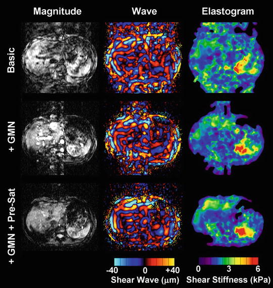
Fig. 3.3
Gradient echo MR elastography with gradient moment nulling and presaturation. This experiment demonstrated that bulk motion can contaminate both the magnitude and wave images and lead to unreliable shear stiffness, as shown in the upper row. The middle row illustrates results implemented with gradient moment nulling. Obviously, the bulk motion was mostly removed from the wave images. To further clean up the motion artifacts from blood flow, presaturation was implemented as well to improve the MRE wave image quality as shown in the bottom row
Intra-Voxel Phase Dispersion
The MEG gradients generate a phase accumulation within an isochromat. In areas of large displacements near the motion source, the phase across an isochromat can begin to disperse. This process is illustrated in Fig. 3.4. The signal dropout can be partially ameliorated by increasing the sampling resolution at the cost of increased breath-hold time. Alternatively, the driver amplitude can be reduced. However this decreases wave penetration and the phase-to-noise ratio. Some signal dropout is an acceptable trade-off to provide sufficient wave penetration into the liver. It is important to exclude these areas of signal void from analysis of liver stiffness.
Fig. 3.4
Magnetization vectors (blue arrows) in the rotating reference frame for a spin isochromat on resonance during application of MRE pulse. (a) Depicts the signal in the complex plane of spins within a voxel not experiencing the effects of motion. As motion increases, the spins begin to dephase (b). Complete signal loss can occur in areas of high motion and the resulting high phase accumulation (c–e) (color figure online)
Alternate Pulse Sequences
Other MRE sequences are available for evaluation of liver stiffness. EPI based Elastography sequences offer significant increases in speed of acquisition over GRE sequences. In multi-slice applications a spin echo implementation, shown in Fig. 3.5, can efficiently sample data for an Elastography study. Patients who have high iron concentration in their liver tissue, which leads to severely, shortened T2*, can be problematic at 1.5 and 3.0 T because it produces poor MR signal in the liver with GRE MRE sequence. Valid stiffness measurements may not be obtained due to the extremely low SNR. Since the signal in SE-EPI sequences experience T2 decay instead of the faster T2* decay, SE-EPI sequences may be an option for patients with high concentrations of iron.
Fig. 3.5
Spin Echo EPI (SE-EPI) pulse sequence. Due to chemical shift artifacts, spatial-spectral pulses are used to generate the initial 90° RF pulse (a). Magnitude and wave images obtained at 3T from a GRE sequence (b) and the SE-EPI sequence (c) show increased signal and better wave depiction obtained with the EPI sequence. Susceptibility artifacts associated with EPI based sequences are not a problem in the liver application
To make the signal further less sensitive to the reduced T2*, which can be as low as ~1.3 ms in iron overloaded liver, a short-TE spin echo and spin echo EPI pulse sequence have been developed and evaluated [56, 57]. The spin echo sequence modification includes fractional MEGs, crusher gradient removal, and split-unipolar MEGs of 2 ms duration positioned on either side of the 180° RF pulse. With these developments, the TE of the sequence could be reduced to 10 ms, and a schematic representation of this sequence is shown in the middle row of Fig. 3.6. In addition to the SE MRE sequence, a spin echo EPI pulse sequence was also developed allowing for faster imaging with modifications similar to the SE MRE pulse sequence. The advantages and disadvantages of EPI-specific parameters including the number of shots and the effective TE were optimized for liver MRE specifically. To achieve the low TE value, chemical presaturation pulses were used instead of a spatial-spectral RF pulse for fat suppression. A schematic of this pulse sequence is shown in the bottom row of Fig. 3.6. Preliminary evaluation of these techniques on both normal volunteers and patients with known iron overloaded liver is very promising [36]. In normal livers, all three sequences provided comparable shear stiffness measurements. In patients, the significant increase of the liver parenchyma signals and high confidence of the calculated stiffness values can be appreciated from SE and SE-EPI MRE sequences.
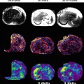
Fig. 3.6
The three pulse sequences and the corresponding MRE data in a patient with iron overload. The GRE technique (top row) failed, but the SE (middle row) and EPI (bottom row) acquisitions provided valid elastograms
STEAM based sequences, seen in Fig. 3.7, are also an option and have been successfully used in cardiac imaging [58, 59]. Most implementations use non-selective hard pulses for the first two RF pulses. This requires a long TR for the signal to recover. However, STEAM Elastography pulse sequences can be efficient in TE. The MEG gradients do not need to be turned on over and entire motion cycle. They can be split and turned on only during a small fraction of the motion cycle.
Fig. 3.7
STEAM sequences inherently split the signal pathways so that only half of the signal is available to sample. The advantage is that T2 decay only occurs during the TE1 and TE2 periods. During the TM period, spins not originating with the first RF can be spoiled with the Gs gradient. Spins following the STEAM pathway will be in the longitudinal plane and will not be affected by the Gs gradient or T2 decay. The MEG gradients are still synchronized to the applied motion however the spins spend much less time in the transverse plan experiencing T2 decay
Slice Selection Criteria for 2-D Liver MRE Acquisition
The MRE visualization of the full 3-D vector displacement field within the liver produced by the passive drivers has proven to offer insights and improvements in both experimental design and 2-D imaging plane selection for in vivo MRE applications [59, 60]. When the results of the 3-D liver MRE acquisition and inversions were used as “ground truth,” 2-D imaging in the “widest” cross-section of the liver consistently yielded inversion results that were comparable to those obtained with the much more time consuming 3-D imaging approach [61]. These studies showed that in a large portion of the liver, the propagation direction of shear waves is approximately parallel with the transverse imaging plane when using a pressure-activated passive driver on the anterior chest wall. This allows accurate elastograms to be generated from 2-D wave image data (which can be acquired in one breath-hold), rather than 3-D wave imaging, which requires longer acquisition times and more complex measures to address respiratory motion. With the acoustic driver system, the 2-D wave approximation is generally valid in the axial imaging planes distanced 2–10 cm away from the superior margin of the liver, assuming the liver has average vertical height of 15 cm. It corresponds to a region across the widest part of the liver as shown in Fig. 3.8. In other marginal levels/regions where the 2-D planar wave model may frequently break down due to special boundary conditions, the shear waves usually traverse obliquely through the plane of interest and may result in erroneous stiffness values.
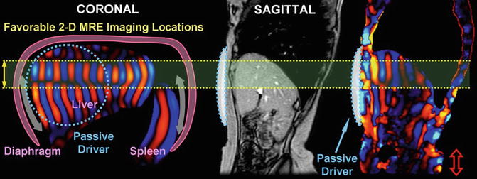
Fig. 3.8
Schematic illustrations of the hepatic MRE setup (with passive driver position indicated) and shear wave generation mechanism (diaphragm act as a secondary driver). Favorable 2-D Liver MRE slice selection locations are indicated in the coronal simulation shown on the right. This was validated in a human study with sagittal imaging locations (motion sensitizing direction is S/I)
Software (Inversion Algorithms)
Dynamic MRE uses propagating mechanical shear waves rather than a static stress as a means to study tissue elasticity. This provides an important advantage for calculating elasticity in that dynamic MRE does not require the estimation of the regional static stress distribution either inside or on the boundaries of the tissue. The acquired wave images are processed using an inversion algorithm to generate quantitative images that depict tissue stiffness, called elastograms. Many different inversion algorithms have been developed to process MRE wave data based on different assumptions about the nature of the wave propagation. Pre-processing algorithms for the wave data include phase unwrapping, removal of concomitant gradient field effects, and directional filtering [62] to enhance the accuracy of the elastograms. Additional pre-processing generates a Background Phase Estimate (BPE) that includes the longitudinal waves, which can be removed to provide the shear wave signal. The inversion algorithms produce stiffness maps using one of the following: measures of the phase gradient or spatial frequency content, direct inversions of the differential equations of motion, or iterative methods involving finite element models [63–67].
The process of generating a stiffness map is achieved by using the MRE displacement data in sliding windows to perform a direct inversion (DI) of the differential equation modeling the wave propagation. A second-order or fourth-order polynomial is fit to the data depending on fit quality. The correlation coefficient (R2) for the fit is recorded for the center pixel of each window. This results in a confidence map with values between 0 and 1, the latter representing high confidence and good signal-to-noise ratio (SNR) [67, 68]. The phase difference wave data obtained from MRE may include the effects of both shear and longitudinal waves. Prior to processing with DI inversion algorithm, an 8-direction motion filters [62] evenly spaced between 0° and 360° and combined in a weighted least-square method to improve the performance of the algorithm are applied, since complex interference of shear waves from all directions may produce areas with low shear displacement amplitude. A BPE is removed from each of the eight directionally filtered data sets. A DI algorithm is then used to estimate the stiffness using the shear wave estimate obtained with each region. SNR map is also obtained using both the magnitude and phase images obtained during the scan. Assuming a constant signal, the magnitude SNR is calculated over a small processing kernel from all the phase offsets. As shown in Fig. 3.9, the phase SNR is obtained with:  Reliability of the liver stiffness measurement at each voxel is then determined by the confidence values from SNR maps.
Reliability of the liver stiffness measurement at each voxel is then determined by the confidence values from SNR maps.Fig. 3.9
Assuming that the MR signal has normally distributed noise in the complex plane, the phase SNR is obtained as a function of arc sin (1/magnitude SNR) and shear wave amplitude. The value is divided by 2, since we gain two factors of  . One
. One  is due to the noise vector being at an arbitrary angle to the signal vector and another
  is from sampling two phase images with opposite gradient polarity and taking their difference (thus adding their signals)
. One is due to the noise vector being at an arbitrary angle to the signal vector and another is from sampling two phase images with opposite gradient polarity and taking their difference (thus adding their signals)All of these steps in processing are done automatically, without human intervention, to yield quantitative images of tissue shear stiffness, in units of kilopascals (kPa). We have used the designation “shear stiffness,” rather than “shear modulus” to indicate that the measurements are effective stiffness values at the driving frequency, and may include a viscous component, although this is likely to be small at the low driving frequency used.
The stiffness maps (elastograms) thus generated include the entire cross-section of the abdomen including the liver and other abdominal organs. Stiffness values can be obtained by placing regions of interest (ROI) on any organ included in that section.
Analysis of Stiffness Maps (ROI Placement for Stiffness Measurement)
The elastograms are analyzed by measuring mean shear stiffness within a large, manually specified region of interest that includes hepatic parenchyma, while excluding major blood vessels, such as hepatic veins, main portal veins, and branches that have width greater than 6 pixels (about 8 mm); liver fissures, gall bladder fossa, and edge of the liver. 2-D liver elastograms are usually calculated based on the assumption of a 2-D planar shear wave field described previously. Ideally, the entire liver parenchyma should be evenly illuminated by planar shear waves with adequate amplitude. However, in practice, the shear waves can be quickly attenuated in the deep structure of the liver; or appear separated in different regions of the liver due to destructive/constructive wave interference at intersections. Therefore, not all hepatic tissue in the final liver stiffness map is measurable. Regions without adequate magnitude signal or shear wave amplitude, which will be identified with the confidence map (as shown in Fig. 3.10), can result in erroneous stiffness value. It is crucial to obtain accurate mean liver stiffness values with appropriate placement of the ROI. Analysis of the liver elastogram should be performed with all original magnitude, phase difference (wave) images, and automatically calculated confidence maps (Fig. 3.10) to ensure that the calculated liver stiffness is reliable.
Get Clinical Tree app for offline access
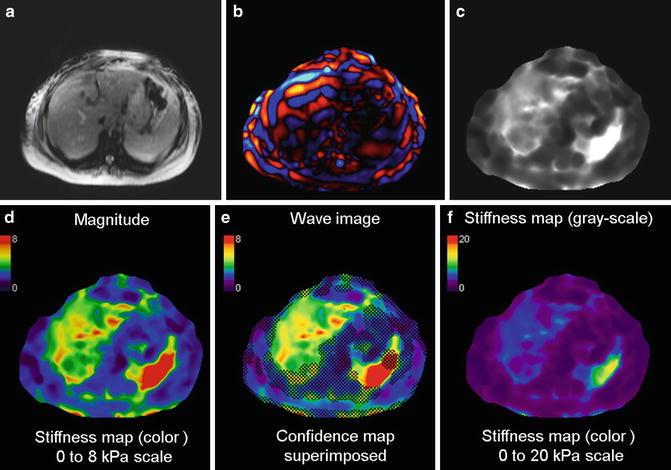
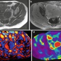
Fig. 3.10
Typical set of images obtained with 2D GRE MRE sequence for a single slice. Magnitude image (a), color phase wave image (b), the gray scale stiffness map (c) on which measurements are obtained, color stiffness map with 0–8 kPa color scale (d), stiffness map with confidence map superimposed (e), and color stiffness map with 0–20 kPa color scale (f
 Introduction
Impact of Magnetic Resonance Elastography on Liver Diseases: Clinical Perspectives
Introduction
Impact of Magnetic Resonance Elastography on Liver Diseases: Clinical Perspectives
 Magnetic Resonance Elastography of the Skeletal Muscle
 Clinical Applications of Liver Magnetic Resonance Elastography: Chronic Liver Disease
 Magnetic Resonance Elastrography of Other Organs
 Magnetic Resonance Elastography of the Lungs


Related posts:
Introduction
Impact of Magnetic Resonance Elastography on Liver Diseases: Clinical Perspectives
Magnetic Resonance Elastography of the Skeletal Muscle
Clinical Applications of Liver Magnetic Resonance Elastography: Chronic Liver Disease
Magnetic Resonance Elastrography of Other Organs
Stay updated, free articles. Join our Telegram channel
Full access? Get Clinical Tree
