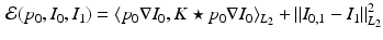
, the LDDMM energy functional is defined as:
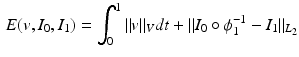
(1)
![$$v \in L^2([0,1], V)$$](/wp-content/uploads/2016/09/A339424_1_En_59_Chapter_IEq2.gif) is a time dependent velocity field drawn from the reproducing kernel Hilbert space (RKHS) V. The RKHS is specified by the choice of kernel K, and the inner product in V is then given by
is a time dependent velocity field drawn from the reproducing kernel Hilbert space (RKHS) V. The RKHS is specified by the choice of kernel K, and the inner product in V is then given by  for any
  . The transformation
  is given by the flow of the velocity v(t, x) through the ODE:
 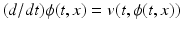 , with initial condition
  . v(t, x) and
  will be written as
  and
and  . The minimizer of (1) is considered the optimal
  for the registration of
  and
and  .
.The second term on the right hand side of (1) is a quantitative assessment of the similarity between the images  and
and  , whereas the first term is the geodesic energy of the flow of
  . For suitable choices of K,
  is always a diffeomorphism [10]; hence, (1) defines
  to be the transformation that best matches
  and
and  such that
  is a geodesic in a space of diffeomorphisms specified by the choice of K. As
  is a geodesic when
  is optimal,
  defines a metric distance
  in the space of diffeomorphisms. This can also be considered a metric
  on the orbit given by the group action of the space of diffeomorphisms on the template image
  .
.
and , whereas the first term is the geodesic energy of the flow of . For suitable choices of K, is always a diffeomorphism [10]; hence, (1) defines to be the transformation that best matches and such that is a geodesic in a space of diffeomorphisms specified by the choice of K. As is a geodesic when is optimal, defines a metric distance in the space of diffeomorphisms. This can also be considered a metric on the orbit given by the group action of the space of diffeomorphisms on the template image .Background, Geodesic Shooting Algorithm: Several approaches to optimizing (1) have been proposed. In this paper we use the geodesic shooting approach [6, 12], which we now review. The kernel K can also be considered a mapping between  , the space of linear functionals on V, and V itself. Note that
  is also a Hilbert space. An Element of
  is called a momentum. Hence for any momentum
  there is some
  such that
  and
and  .
.
, the space of linear functionals on V, and V itself. Note that is also a Hilbert space. An Element of is called a momentum. Hence for any momentum there is some such that and .An optimal solution to (1) specifies a geodesic, which is uniquely determined by its initial velocity  , or equivalently, its initial momentum
  .
.  for all t, and hence
  and
and  , can then be determined by solving the co-adjoint equation [6]:
  , where D denotes the Jacobian operator and div(.) the divergence operator. If the initial momentum is assumed to be proportional to the template image gradient, that is
 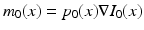 for some scalar field
  , the adjoint equation can be separated into a disjoint system of differential equations for
  and
and  respectively [12], where
  . Considering these equations and the gradient of (1) with respect to
  , we arrive at a system of partial differential equations that completely specifies
  given initial conditions
  and
and  (
( denotes convolution):
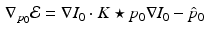
With this in mind, (1) is replaced with a functional of the initial momentum exclusively:
and optimization proceeds within  only. In order to optimize (3) by gradient descent, we need the gradient of (3) with respect to
  , subject to the geodesic shooting constraints (2). This naturally gives way to an optimal control problem. Time dependent Lagrange multipliers
  ,
,  , and
, and  enable us to write an augmented functional for (3) incorporating the constraints (2):
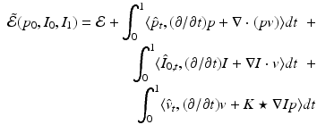
The first variation of (4) gives the gradient of (3) subject to (2):
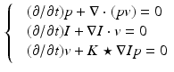
where  is specified by a system of partial differential equations solved backward in time termed the adjoint system:
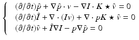
with initial conditions  and
and  . The gradient descent proceeds by solving the system (2) forward in time to acquire
  ,
,  , and
, and  for a sufficiently dense sampling of
 ![$$t \in [0,1]$$](/wp-content/uploads/2016/09/A339424_1_En_59_Chapter_IEq62.gif) , then solving (6) backward in time to acquire
, then solving (6) backward in time to acquire  .
.  is then updated with (5), and the process is repeated until convergence.
, or equivalently, its initial momentum . for all t, and hence and , can then be determined by solving the co-adjoint equation [6]: , where D denotes the Jacobian operator and div(.) the divergence operator. If the initial momentum is assumed to be proportional to the template image gradient, that is for some scalar field , the adjoint equation can be separated into a disjoint system of differential equations for and respectively [12], where . Considering these equations and the gradient of (1) with respect to , we arrive at a system of partial differential equations that completely specifies given initial conditions and ( denotes convolution):(2)
(3)
only. In order to optimize (3) by gradient descent, we need the gradient of (3) with respect to , subject to the geodesic shooting constraints (2). This naturally gives way to an optimal control problem. Time dependent Lagrange multipliers , , and enable us to write an augmented functional for (3) incorporating the constraints (2):(4)
(5)
is specified by a system of partial differential equations solved backward in time termed the adjoint system:(6)
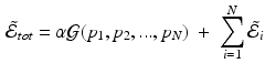
and . The gradient descent proceeds by solving the system (2) forward in time to acquire , , and for a sufficiently dense sampling of , then solving (6) backward in time to acquire . is then updated with (5), and the process is repeated until convergence.Group-wise Similarity Prior: We consider the case where we are given N longitudinal image pairs 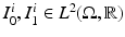 ,
, ![$$i \in [1,2,...,N]$$](/wp-content/uploads/2016/09/A339424_1_En_59_Chapter_IEq66.gif) , all taken approximately the same time interval apart. We take
, all taken approximately the same time interval apart. We take  to be the unit cube with periodic boundary conditions, and the time interval to be [0, 1]. Additionally, we are given N transformations
  mapping the initial images
  to a Minimal Deformation Template (MDT) coordinate system, that is,
 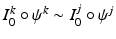 for all k and j. To consider all N registrations simultaneously with no modification to the geodesic shooting approach, we could write
  where
where  is eq. (3) for the ith image pair. The first variation of
  with respect to an initial momentum
  will only include terms for the ith pair, that is, the N transformations are decoupled. However, we would like the N transformations to explore the space of diffeomorphisms as a group. We couple them by considering equations of the form:
 is intended to enforce some criteria that we may think all
  must satisfy. In this paper, we consider longitudinal studies where all N image pairs come from patients in the same diagnostic group, where a predictable distribution of volume change is known to occur. Because
  is a Hilbert space, we can calculate statistical moments in this space in an ordinary manner, being careful to spatially normalize the
  to a MDT coordinate system using coadjoint transport [15]. First, let
 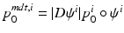 , be the ith initial momentum in the MDT coordinate system. Let
 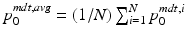 be the sample average initial momentum in MDT coordinates. Let
 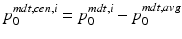 be the mean centered initial momentum for image pair i in MDT coordinates, and let
 ![$$A = [p^{mdt,cen,1}_0, p^{mdt,cen,2}_0,...,p^{mdt,cen,N}_0]^T$$](/wp-content/uploads/2016/09/A339424_1_En_59_Chapter_IEq82.gif) be the mean centered design matrix for all initial momenta in MDT coordinates. We take
be the mean centered design matrix for all initial momenta in MDT coordinates. We take  to be:
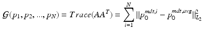
the trace of the sample inner-product matrix for  .
.
, , all taken approximately the same time interval apart. We take to be the unit cube with periodic boundary conditions, and the time interval to be [0, 1]. Additionally, we are given N transformations mapping the initial images to a Minimal Deformation Template (MDT) coordinate system, that is, for all k and j. To consider all N registrations simultaneously with no modification to the geodesic shooting approach, we could write where is eq. (3) for the ith image pair. The first variation of with respect to an initial momentum will only include terms for the ith pair, that is, the N transformations are decoupled. However, we would like the N transformations to explore the space of diffeomorphisms as a group. We couple them by considering equations of the form:(7)
is intended to enforce some criteria that we may think all must satisfy. In this paper, we consider longitudinal studies where all N image pairs come from patients in the same diagnostic group, where a predictable distribution of volume change is known to occur. Because is a Hilbert space, we can calculate statistical moments in this space in an ordinary manner, being careful to spatially normalize the to a MDT coordinate system using coadjoint transport [15]. First, let , be the ith initial momentum in the MDT coordinate system. Let be the sample average initial momentum in MDT coordinates. Let be the mean centered initial momentum for image pair i in MDT coordinates, and let be the mean centered design matrix for all initial momenta in MDT coordinates. We take to be:(8)
.First we consider the rightmost form of (8). We see that this term maintains a group-wise average of the initial momentum, and requires that all momenta be close to this average. This is similar to hierarchical latent variable models that maintain a group-wise representation of the data and constrain updates to predictions to be similar to this representation.
Related posts:
 Stable Overlapping Replicator Dynamics for Multimodal Brain Subnetwork Identification
 PET Reconstruction with Sparse Image Representation and Anatomical Priors
Stay updated, free articles. Join our Telegram channel

Full access? Get Clinical Tree


