(1)
Department of MRI, Medical Center at Siegerland Airport, Burbach, Germany
We have taken a look at the construction of MRI systems, how they work, and which low-field-specific aspects of physics have to be considered. Now, before we consider clinical imaging, we will think about ways to optimize low-field scanning, which advantages we can use and which drawbacks we have to be aware of.
6.1 Positioning
Let us start with the patient itself. The patient is one important source of artifacts: body movement, breathing, heartbeat, vessel movement, and bowel peristalsis.
The best patient is one who feels comfortable and relaxed, experiences no pain, and maybe has something to hear (music) or look (pictures) at.
Very important is the effect of a large daylight window, visible from the patient table (see Sect. 3.9).
Permanent magnets allow an open design, providing good access to the patient, reduce claustrophobia, and ease positioning. This improves comfort for patient as well as healthcare professionals. Comfort means better compliance of the patient, better imaging results by reduced motion, and better tolerance, even if the patient suffers from claustrophobia (Rothschild et al. 1992; Heuck et al. 1997; Hayashi et al. 2004).
In certain clinical situations, it may also mean increased safety. This is regularly the case in patients who need intensive care. Positioning is far more easy. The anesthesiologist has nearly free access to the patient. Possible missile effects of ferromagnetic medical devices are significantly reduced (Kaufmann 1989; Bohinski et al. 2001).
Comfortable patient positioning is a crucial prerequisite for successful imaging. Furthermore, it is important that the patient understands the examination procedure. It is good practice to explain to the patient what will happen and how long the examination takes. We tell the patient that this machine is very careful with his body and that we therefore have to invest some more time in the examination. If ever possible, we talk to the patient during the procedure – talking makes it easier for the patient and gives us a kind of “interactive biomonitoring.”
6.2 Sequences
In this section, we will briefly address the sequence technique and consider low-field-specific changes of the scan procedure.
6.2.1 Spin Echo
Spin echo sequences are the classical “working horses” of MRI.
1.
The sequence starts with a 90° RF excitation pulse. The gradient in z-direction is switched on.
2.
The phase encoding gradient is switched on.
3.
After a time TE/2, a 180° inversion pulse is transmitted.
4.
The readout gradient is switched on. The spin phase is different for each phase encoding step.
5.
After a time, TE the spins are in phase again, giving the maximum spin echo.
6.
After recovery of the z-magnetization, the next sequence is started (Fig. 6.1).
Fig. 6.1
Spin echo sequence pulse sequence timing diagram
Sequences with a short echo time TE (minimal TE, about 15 ms) and a short TR (400–600 ms) are influenced mainly by T1 relaxation. Short TE, long TR gives a proton-density image. Long TE, long TR results in images influenced more by T2 relaxation.
The shorter T1 time at lower-field strength provides higher signal at short TE and a better T1 contrast.
Minimum TE is depending on the gradient performance in terms of gradient amplitude and, more importantly, gradient slope (or rise time). The combination of these two parameters is called “slew rate.”
Some younger low-field scanners have improved gradient performance.
A good example is gradients with 24 mT/m amplitude and a rise time of 450 ms. The slow rate is therefore 55 T/m/s, enabling sufficiently short echo time.
Since T1 relaxation is faster, the time until recovery of longitudinal relaxation is completed is shorter: TR can be reduced to <500 ms, providing some gain in scan time, at equal signal-to-noise and contrast-to-noise ratio (SNR and CNR).
T2-weighted sequences do not take profit from lower field strength, contrast-enhanced T1 sequences likewise, due to the reduced contrast effect of Gd (see below).
6.2.2 Multi-Spin Echo
To increase scan speed, one excitation pulse can be followed by multiple inversion pulses (multi-echo). The higher the number of echoes/TR, the faster is the sequence. Since TR is short in T1 sequences, they take only limited profit. For T2 sequences with long TR, the number of echoes can go up to 100/TR and above. The late echoes, however, have lost most of their signal (Fig. 6.2).
Fig. 6.2
Fast spin echo pulse sequence timing diagram
To increase signal strength for sequences with long echo trains, a trick is played: The early echoes fill the central part of the signal space (k-space) defining image contrast. The late echoes fill the peripheral part of the k-space, giving mainly contour information (Fig. 6.3).
Fig. 6.3
(a) Central k-space contains contrast information. (b) Peripheral k-space contains contour information
Peter Rinck gives a beautiful example for the k-space function (Rinck 2009) (Fig. 6.4)

Fig. 6.4
A cat by day, and a cat by night. In bright daylight, the pupil is small, the central parts of the retina give excellent resolution. At night, the pupil widens, since the peripheral parts of the retina are needed to gain as much of the weak light (signal) as possible
6.2.3 Gradient Echo
In a gradient echo sequence, spin rephasing is not achieved using an inversion 180° RF pulse, but by inverting the frequency encoding gradient. Keep it simple! (Fig. 6.5)
Fig. 6.5
Gradient echo pulse sequence timing diagram
Since there is no time needed for an echo refocusing pulse, TE can be shorter, and therefore, gradient echo sequences are better suited for shorter T1 times in low-field imaging.
A big drawback of gradient echo is the strong influence of gradient field inhomogeneities, particularly in T2 images. These are compensated, if the spins “go back the same way they came” after a refocusing RF pulse. Therefore, T2-weighted images in gradient echo sequences are addressed to as T2* images.
Further inhomogeneities occur through susceptibility effects, causing areas of rapid dephasing, black ribbons, on bone–fat or bone–air borders (paranasal sinus). To reduce this additional T2* effect, short T1 times are preferred, again supporting the advantages of low-field scanners.
Susceptibility effects are used to detect small iron deposits in areas of micro-hemorrhage (sequence names: GE, SWAN; Siemens, HEMO).
6.2.4 Rapid Gradient Echo Imaging
One way to increase the scan speed of gradient echo sequences is to reduce the proton flip angle. The excitation pulse is selected <90°. Therefore, only a part of the protons is flipped. Since TR is short, the residual z-magnetization increases the signal for the next excitation pulse. Haase and coworkers invented this technique in 1986 and called it FLASH (fast low-angle shot) (Haase et al. 1986). The optimal “flip angle,” yielding maximum signal, is called the Ernst–Winkel.
![$$ \mathrm{Ernst}-\mathrm{Winkel}={ \cos}^{-1}\left[ \exp \left(-\mathrm{T}\mathrm{R}/\mathrm{T}1\right)\right] $$](/wp-content/uploads/2016/10/A329734_1_En_6_Chapter_Equa.gif) Therefore, with shortened T1 times in low-field imaging, larger flip angles are possible (Fig. 6.6).
Therefore, with shortened T1 times in low-field imaging, larger flip angles are possible (Fig. 6.6).
Fig 6.6
In gradient echo sequences, the flip angle (α) is important for T1-weighted images. GE sequences generally use small flip angles (<90°) and very short TRs (typically 150 ms). The optimal flip angle depends on the T1 value of the tissue being imaged. A short T1 results in a larger optimal flip angle. Dotted line: best contrast-to-noise ratio for a TR of 100 ms
In the late 1970s, Peter Mansfield had a brilliant idea (Mansfield and Maudsley 1977). A single excitation pulse, followed by a series of strong gradients, resulting in a series of gradient echoes (echo train) (Fig. 6.7).
Fig. 6.7
Echo planar imaging pulse sequence timing diagram
This extremely fast imaging is strongly influenced by susceptibility effects. Today, it is mainly used for diffusion-weighted imaging (Fig. 6.7).
EPI imaging takes advantage from higher field strength and gradient performance. Therefore, on low-field scanners, it is possible, but less frequently used. There are concerns about safety of EPI imaging: The rapid gradients can cause eddy currents, potentially leading to neuromuscular stimulation.
If multiple gradient echoes are acquired (fast gradient echo), a further increase of speed is possible. The problem is incomplete recovery of magnetization. Different approaches are realized:
Refocusing the magnetization with an RF pulse (FISP, FFE).
Spoiling the residual magnetization with a spoiler gradient at the end of the read out (FLASH, GFE).
Balanced scanning: The sequence contains two RF excitation pulses. Before the second pulse, the gradients are balanced, so their net value is zero; all spins are excited by the second RF pulse (True-FISP, FIESTA).
Ultrafast gradient echo uses extremely short TE (2 ms) and TR (3–5 ms); the flip angle is about 5°, giving poor tissue signal. Acquisition time is <1 s.
A 180° inversion pulse starts the sequence, giving the option to use the zero passing and selectively suppress fat or water or silicone (breast imaging).
The readout module may use a single shot (excitation) with variable flip angle or multiple segments (multi-shot). If multiple lines are acquired after a single pulse, the pulse sequence is a type of gradient echo planar imaging (EPI) pulse sequence (Fig. 6.8).
Fig. 6.8
Ultrafast gradient echo pulse sequence timing diagram
6.2.5 3D Imaging
The first MRI examinations in the late 1970s and early 1980s were three-dimensional sequences. The larger the excited volume, the smaller the noise component. Therefore, 3D imaging has a much better SNR than 2D imaging. A 3D sequence is produced by applying an RF excitation pulse without slice selection gradient to a regular 2D sequence, exciting the whole imaging volume.
The disadvantage is the long examination time, which made gradient echo sequences the typical 3D technique.
In 2007, Erik Schweitzer made a far seeing statement during David Stoller’s course on musculoskeletal MRI. He said that in maybe 10 years, an MRI could be performed with only one 3D turbo spin echo sequence. It didn’t take 10 years, but it was a close guess.
A regular fast (turbo) spin echo sequence with an echo train (turbo factor) of 20 and 256 × 256 matrix and 128 slices (the interlacing slice is interpolated to get an isometric volume) takes at a TR of 2.5 s 68 min. Using parallel imaging, this can be shortened to 34 min. Still too long for clinical routine.
The newest 3D TSE sequences (Dr. Schweitzer was right) are called SHAPE in the Siemens world, VISTA on Philips, and CUBE on GE machines. They have an echo train length of >100. With such a long ETL, there is usually only very few signal left for the late echoes. This signal has to be increased.
A possible trick is a refocussing pulse with variable reduced flip angle. Flip angles below 180° lead to reduced early echo intensities but conserve more signal for the late echoes. The original name was FSE-XETA (fast spin echo with extended echo train acquisition) (Fig. 6.9).
Fig. 6.9
(a) Refocussing with a 180° pulse results in weak late echoes. (b) Reduced angle preserves more signal. (c) Modulated angle can result in even stronger late signal
Another trick is a three-dimensional reconstruction kernel for parallel imaging using self-calibration and a three-dimensional interpolation of missing data. The algorithm is called ARC (Autocalibrating Reconstruction for Cartesian imaging) (Fig. 6.10).
Fig. 6.10
ARC. A three-dimensional data space is partially filled with measured data. The missing data are computed by 3D interpolation, reducing the needed scan information
The resulting 3D TSE sequence is able to scan a T2-weighted sequence with a TR of 2.5 s, an ETL of 100, and a 256 × 256 × 256 volume in 4:30 min. The RF power is low, with metal artifacts reduced. SNR and tissue contrast are spin echo like.
These sequences can be performed on low-field scanners with a to some extent longer scan time (due to less SNR).
6.2.6 Fat Saturation
Fat is bright in T1, T2, and proton-density imaging. Contrast enhancement results in signal increase in pathologic (inflammatoric, neoplastic, hyperperfused) areas. Edema is bright in T2-weighted sequences. To increase detectability of these pathological findings, the suppression of bright fat signal is mandatory.
Different concepts and techniques exist for fat suppression. Since field strength has an important effect on fat suppression effects, they have to be briefly addressed.
There are two principles for fat suppression: relaxation dependent (STIR) and chemical shift dependent (Dixon, spectral saturation, water excitation, and SPAIR) (Horger and Kiefer 2011).
6.2.6.1 Dixon Technique
In 1984 W.T. Dixon proposed a novel technique for fat saturation in MRI (Dixon 1984).
This technique makes use of different resonance frequencies (chemical shift) of fat and water-bound protons. Basically, two images are acquired: an image where the fat and water protons are “in-phase” and an image where fat and water protons are “opposed-phase.” Four contrasts can be provided: fat image, water image, “in-phase” image, and “opposed-phase” image.
Since a long TR is required to obtain these scan data, the scan time is relatively long, which can be partially compensated by parallel imaging (Wohlgemuth et al. 2002).
The Dixon technique is well suited for low-field systems and can represent an alternative to spectral fat saturation techniques in high-field settings.
6.2.6.2 Spectral Fat Saturation
For the chemical shift between fat and water protons, the difference in resonance frequency is 3.4 ppm. Spectral fat saturation uses this frequency difference by emitting a narrow band pulse at the fat frequency, switching fat protons off the z-axis direction (and deleting the resulting transverse magnetization by spoiler gradients).
Since the frequency offset is proportional to field strength, it is markedly reduced in low-field MRI (66 Hz at 0.4 T, see above).
Two modes of fat saturation intensity can be selected (strong/weak), defining how much signal the fat-bound protons contribute to the image.
Spectral fat saturation does not affect tissue contrast and is therefore frequently used. It is depending on homogeneity of the B o and B 1 field. The additional preparation pulses increase scan time.
Therefore, to achieve sufficient image quality in spectral saturated sequences on a low-field MRI is challenging.
6.2.6.3 Water Excitation
Fat suppression by spectral saturation costs signal. An alternative is to selectively excite the water-bound protons.
This means, no additional pulses are needed, but the minimum TE is longer. The sequence is less dependent from B 1-field inhomogenieties, which is more important for 3 T scanners.
6.2.6.4 STIR
The acronym means “short TI inversion recovery”. Fat has a shorter T1 relaxation time than other body tissues. Before the scan sequence, a 180° inversion pulse is applied, which flips all spins in the –z-direction. This is followed by T1 relaxation. After a time TIfat, the fat protons are in transverse orientation. If the 90° excitation pulse is emitted at this time, the fat protons cannot contribute to the resonance signal. This process is called “zero passing.”
STIR images have an inverted T1 contrast (not T2 contrast).
In principle, the fat zero passing is reached when
 In practice, the optimal value will also depend on other sequence parameter settings (e.g., TR); the typical TI at 1.5 T is chosen to be 150 ms. TI will also depend on field strength since T1fat increases with field strength. If the TI value is selected <150 ms, more fat signal is received, reducing fat suppression, but improving image signal to noise.
The major advantage of STIR imaging is the complete insensitivity to B 0 inhomogeneities. Furthermore, it doesn’t depend on chemical shift. This predestines this technique for fat suppression in areas with signal and field inhomogeneity, like shoulder or foot.
One major disadvantage is that it cannot be used after intravenous contrast injection. Gd shortens the T1 time of all tissues, which can then have the same “zero-passing” time as fat. The other disadvantage is the reduced SNR compared with spectral saturated spin echo sequences (see above).
6.2.6.5 SPAIR
The acronym stands for “spectral adiabatic inversion recovery.” Different from STIR, only the fat protons are inverted by a 180° pulse. With gradient spoiling, the transverse magnetization is deleted. The inversion time TI is selected at the time, when the contribution of fat-bound protons to the signal is nulled.
Since this sequence uses a frequency selective inversion, it is not well suited for low-field scanners (Horger and Kiefer 2011).
For musculoskeletal imaging, spectral fat saturation in proton-density images is optimal for evaluation of cartilage lesions. For MR arthrography, regular T1-SE sequences with spectral fat saturation are used. For the latter application, a contrast-enhanced MR angiography sequence or a DIXON fat saturation technique is a possible alternative (ultrafast short TE 3D gradient echo).
What works best and most reliable for fat suppression is STIR imaging. Since STIR is strongly T1-dependent, high-resolution images are provided, sensitive for bone marrow edema and even for cartilage surface evaluation (Fig. 6.11).
Fig. 6.11
(a) STIR pulse sequence timing diagram. A 180° preparation pulse skips the spins in –z-direction. (b) At a time TI of 150 ms (1.5 T) fat protons and at a time TI of 2200 ms (1.5 T), free water protons are in the transverse plane and do not contribute to signal. This allows a reliable suppression of fat or water
6.2.7 Diffusion Imaging
Diffusion imaging uses the movement of water molecules as contrast-giving principle. Different sequence types are used.
Basically, it is a T2-weighted spin echo, gradient echo, or EPI sequence, using a 180° – rephasing pulse surrounded by a bipolar gradient pair of equal strength. This means that movements between this gradient pair are not completely rephased, which leads to a signal loss. The signal loss is proportional to the spin movement, which in turn depends on the presence of diffusion barriers, like cell membranes. In case of disease (tumor, ischemia), the cell membranes can be damaged, which leads to increased diffusion.
sensitivity of measurement concerning diffusion is based on strength and duration of the gradient pair, as well as the time interval between the gradient activation. These conditions are summarized in a “sensitivity coefficient” b, given by
 with γ = gyromagnetic constant of hydrogen, G = strength of diffusion gradient, δ = duration of the gradient, and Δ = time interval between the gradient. The higher the value, the higher the signal loss by diffusion of water molecules.
Related posts:


Stay updated, free articles. Join our Telegram channel

Full access? Get Clinical Tree


