Magnetic Resonance Elastography of the Heart

(10.1)

${\sigma}_{\mathrm{m}}=P\left(\frac{V}{V_{\mathrm{w}}}\right)\left(1+\frac{b^3}{2{R}^3}\right)$

(10.2)

where σ _m = stress at the mid wall, V = volume of the chamber (i.e., LV cavity), V _w = volume of the wall (remains constant as the material is assumed to be incompressible), P = internal cavity pressure (i.e., chamber pressure), a = inner radius of the shell, b = outer radius of the shell, R = (a + b)/2 (i.e., mid wall radius), and dP/dV = chamber stiffness [1, 2].

Fig. 10.1

Measurement of the EDPVR requires creating a family of pressure–volume (PV) loops, which are obtained by simultaneously measuring pressure and volume at different loading conditions. End-diastolic pressure points are plotted to create the EDPVR curve, the slope of which is an estimate of chamber stiffness. In these hypothetical PV loops, the end-systolic points have also been plotted to obtain the end-systolic pressure volume relationship (ESPVR), the slope of which is E _es. Reprinted from Burkhoff et al. [1]

Because the EDPVR is non-linear, there are a variety of curves to which it may be fit and there is currently no consensus regarding which is the most accurate.

MRE Pulse Sequences for Cardiac MRE Applications

Accurate assessment of myocardial stiffness using MRE-based methods is challenging. Respiratory induced bulk motion as well as the volumetric changes of the heart’s chambers as they expand and contract throughout the cardiac cycle violate the assumptions imposed on existing MRE inversion algorithms and thus can produce erroneous estimates of myocardial stiffness. The unique geometry of the heart also means that wave propagation cannot be described as a plane shear wave propagating within an infinite medium. Without appropriate modeling of the boundary conditions imposed by the geometry of the heart and the resultant effect on wavelength, erroneous assessment of myocardial stiffness can result. The following discussion describes the various methods under development to address these challenges.

Advanced Geometric Modeling of the Left Ventricle

Due to the unique geometry of the heart—four thin walled fluid filled cavities that undergo cyclic changes in wall thickness and volume—several underlying assumptions imposed by commonly used inversion algorithms become invalid and therefore create the potential for incorrectly estimating myocardial stiffness. To improve the accuracy of this estimate, it is necessary to develop inversion algorithms that more closely model the heart’s physical characteristics. When vibrations from an external source are introduced into an object in which the wavelength of the vibration is greater than the thickness of the object, flexural (i.e., bending) waves are generated. Kolipaka et al. [3] have investigated flexural waves in bounded media such as thin beams, plates, and spherical shells as potential models for visualizing vibrations below several hundred Hertz within the myocardium from a passive longitudinal driver such as those used in clinical MRE studies to more accurately assess myocardial stiffness. Because spherical shells most closely match the geometry of the chambers of the heart, only this model will be presented.

When vibrations are introduced into a spherical shell, flexural waves are generated as a result of the shell’s boundary conditions. By application of Hamilton’s variation principle with the assumption of mid surface deflections and non-torsional axisymmetric motion, the equations of motion of these waves can be solved to provide an estimate of the flexural motion and are given in the equation below [3] assuming that; (1) the displacement of the shell is small in comparison to its thickness, (2) the thickness of the shell is small compared with the smallest radius of curvature, (3) “fibers” or elements of the shell initially perpendicular to the middle surface remain so after deformation and are themselves not subject to elongation, and (4) the normal stress acting on planes parallel to the shell middle surface is negligible in comparison with other stresses.

$\begin{array}{l}\begin{array}{l}{\beta}^2\frac{\partial^3u}{\partial {\theta}^3}+2{\beta}^2 \cot\;\theta \frac{\partial^2u}{\partial {\theta}^2}-\left[\begin{array}{l}\left(1+\nu \right)\left(1+{\beta}^2\right)\\ {}\kern0.6em +{\beta}^2{ \cot}^2\theta \end{array}\right]\frac{\partial u}{\partial \theta}\\ {}+ \cot\;\theta\;\left[\left(2-\nu +{ \cot}^2\theta \right){\beta}^2-\left(1+\nu \right)\right]u-{\beta}^2\frac{\partial^4w}{\partial {\theta}^4}\end{array}\hfill \\ {}\begin{array}{l}-2{\beta}^2 \cot\;\theta \frac{\partial^3w}{\partial {\theta}^3}+{\beta}^2\left(1+\nu +{ \cot}^2\theta \right)\frac{\partial^2w}{\partial {\theta}^2}\\ {}-{\beta}^2 \cot \theta\;\left(2-\nu +{ \cot}^2\theta \right)\frac{\partial w}{\partial \theta }-2\left(1+\nu \right)w\\ {}-\frac{a^2\ddot{w}}{c_p^2}=-{p}_a\frac{\left(1-{\nu}^2\right){a}^2}{Eh}\end{array}\hfill \end{array}$

(10.3)

This equation provides an estimate of Young’s modulus, E from which the shear modulus can be obtained by substation in the equation μ = E/2(1 + v) where v is the Poisson’s ratio of the material.

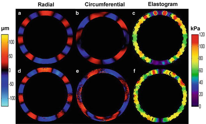
Figure 10.2 shows both simulation and experimental displacement maps for the radial and circumferential components of the flexural wave resulting from the application of a sinusoidal force at a frequency of 200 Hz to the top surface of a thin silicone rubber spherical shell of 10 cm diameter and thickness of 1 cm. The in-plane components of displacement were encoded using a gradient-echo MRE sequence with 5 ms duration MEG. The third column of this figure shows the reconstructed map of shear modulus (i.e., the elastogram). There are several reasons for the relative heterogeneity of the elastogram images including the sensitivity of the above equation of motion to noise as a result of the third order derivatives as well as the singularities at the two poles of the shell (θ = 0° and 90°). Despite these sources of error, the model is able to provide an accurate estimate of shear stiffness which has been validated using finite element modeling simulations and is shown in Fig. 10.3.

Fig. 10.2

Shear wave displacement images of a thin spherical shell undergoing mechanical excitation for both finite element modeling simulations (a, b) and MRE experiments (d, e), respectively, for a 1 cm thick shell vibrated at a frequency of 200 Hz. (c, f

Only gold members can continue reading. Log In or Register to continue