MAGNETIC RESONANCE IMAGING: INTRODUCTION AND GENERAL PRINCIPLES
This chapter is dedicated to the memory of E. Raymond Andrew, PhD
KEY POINTS
- Basis of magnetic resonance relaxation processes
- Basis of magnetic resonance imaging spatial resolution
- Basis of magnetic resonance imaging contrast resolution
- Fat-suppression imaging
- Flow-related issues and imaging
- Diffusion-weighted imaging
- Intravenous paramagnetic contrast use
- Effects of magnetic susceptibility
- Factors affecting protocol development and imaging strategy choices in clinical practice
- Speculative value of magnetic resonance spectroscopy
Basic magnetic resonance imaging (MRI) physics is the foundation for understanding how to use this imaging tool to its fullest advantage. There are many excellent sources for a complete discussion of this principle knowledge base. The following discussion assumes that much of the basic foundation of MRI physics is known to the reader. However, some basic physics is presented in summary form to emphasize the rational basis for the protocol development and image interpretation.
MRI is based on the knowledge that biologic tissue is permeable to long wavelengths such as that of the electromagnetic radiation used for magnetic resonance (MR). When immersed in a very strong magnetic field, nuclei possessing a spin are capable of absorbing energy from radiofrequency (RF) waves thereby temporarily transitioning to higher energy levels. According to their molecular configurations and physical state, nuclear spins will transition back to their original energy levels at different rates. The difference in these rates is what ultimately generates contrast in an MR image. Basically, the MR device is capable of collecting and interpreting this information about the nuclei transitioning back to their ground states. Different system configurations can determine how these signals are generated and collected and thus how they affect image quality. Major variations in system performance are influenced by differences in the receiver design, direction of the magnetic field relative to the long axis of the body, and magnetic field strength. Acceptable basic head and neck imaging can be done at fields of 0.2 to 0.5 Tesla (T) for some indications. The best spatial resolution is attained at ≥1 T, and there may not be any clinically essential improvement in spatial resolution between 1.5 and 3.0 T for extracranial indications. Certainly, the signal-to-noise ratio (SNR) improves for increased field strength; however, there are ways to compensate for differences in field strength so that the basic diagnostic information may be available at all fields in optimized systems operating from about ≥0.2 T. An exception to this rule is the information resulting from magnetic susceptibility differences such as that induced by blood products. Magnetic susceptibility effects, discussed in more detail later in this chapter, are routinely visible on 0.15- to 0.50-T instruments but are much better observed at higher fields. Gradient-recovered echo (GRE) techniques can be used to overcome some of this disparity. Higher field systems (≥1.0 T) present more losses as a result of physiologic motion, tuning difficulties, coil-loading effects (Fig. 3.1), and chemical shift (Fig. 3.2). These losses or artifacts are expressed more in body imaging but are present in extracranial head and neck imaging.


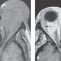
FIGURE 3.1. T1-weighted fat-suppressed images of the neck demonstrating lack of homogeneity of fat suppression. A: A section through the low neck at the junction of the neck and thoracic inlet shows extremely inhomogeneous fat suppression mainly in the anterior portion of the neck and some more posteriorly. B: Image somewhat higher showing relatively homogeneous fat suppression in the area of interest but still relatively poor fat suppression posteriorly. The latter is not a diagnostic problem. (NOTE: The unreliable nature of frequently selective fat suppression when applied to regions where there is differential loading of the receiver coil makes this technique inherently somewhat unreliable. The main problem in head and neck imaging is at the junction of the neck and chest.)

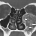
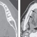
FIGURE 3.2. T2-weighted non–fat-suppressed image of the orbit showing chemical shift artifact (arrows).
Optimal image quality at all field strengths requires the best system design, specifically including system electronics that decrease system noise and receiver side design that carefully matches coils and couples them closely to the anatomic area of interest. Other options, such as improving slice-selective RF pulse shapes, fat suppression (FS), motion compensation, fast spin echo (FSE) techniques, and parallel processing are available on most systems. Imaging at lower fields will always result in a compromise of image quality as compared with imaging at higher (≥1 T) fields; thus, it is a primary responsibility of the head and neck radiologist to advise the referring clinician about the magnitude of that risk in that particular patient and diagnostic situation. This will help assess whether the confidence level in the imaging findings will match with an acceptable risk of a missed diagnosis because of image quality limitations. In general, many applications of head and neck MRI should not be done under 1 T by choice.
If the MR system is optimized, certain limitations on the basic imaging parameters, mainly related to voxel size, will be imposed on the basis of field strength alone. This basic concept of SNR/voxel was discussed in Chapter 1. Increased signal averaging at lower fields can help to overcome some loss of SNR at the expense of increased imaging time.
SPATIAL RESOLUTION
The basic concepts of the voxel and the relative impact of image contrast, spatial resolution, and SNR on image quality were introduced in Chapter 1. The interrelationships of these factors are fundamental to the understanding of the following discussion.
The spatial resolution requirements determine in part the lower limits of acceptable SNR in any imaging system. In MRI, when voxel size is decreased, the number of protons per voxel decrease. When slice thickness (SLT) is narrowed, the effect is linear so that one-half the SLT results in one-half the protons in the voxel and one-half the original signal. When pixel size is reduced (field of view [FOV] decreased), the size decrease is in two dimensions so that halving the pixel dimensions diminishes the SNR by a factor of 2.8. Considering these profound effects of decreasing voxel size on SNR, one can begin to realize the trade-off in balancing the needs of spatial resolution and image contrast when deciding on pulse sequence protocols for a particular region of interest.
In the first decade of MRI, the existing T2-weighted (T2W) spin echo (SE) techniques necessary to produce contrast between normal brain and intra-axial pathology required a long pulse repetition time (TR), which, in the interest of shorter total acquisition times, limited the amount of signal averaging possible through sequence repetition to make up for the signal loss if smaller voxels were desired. The corresponding longer echo time (TE) required in the same T2W sequences results in lower signals in each voxel because the transverse tissue magnetization has decayed considerably by the time it was sampled, further aggravating the low SNR per voxel problem. With the coming of high fields, there was enough SNR per voxel to allow the SLT to be within the 3- to 5-mm range and the FOV in the 14- to 20-cm range, respectively, on T2W SE images if a quadrature head coil were used. However, at lower field strengths, the slices had to be thicker and the FOV larger to produce voxels of sufficient size to generate an image of acceptable quality. This limitation was essentially overcome to a large extent with FSE techniques that revolutionized MRI with respect to balancing spatial resolution needs on T2W sequences even at lower field strengths.
The basic physics of GRE, FSE, and the “ultra-fast” echo planar imaging (EPI) methods are available elsewhere. GRE and FSE techniques are now generally available in all scanners. The value of GREs for susceptibility-weighted imaging is discussed later in this chapter in the section on relaxation. A single slice, breath-holding, rapid (i.e., computed tomography [CT]–like) acquisition suitable for routine use is not yet available for the extracranial head and neck; this is mainly due to the susceptibility artifacts encountered at air–bone interfaces and those due to dental fillings and metal devices. Vascular imaging with SE and GRE techniques are discussed in the section on magnetic resonance angiography (MRA).
FSE techniques have been in clinical development since about 1990 and were introduced to the general user in 1992. The first technique to be released was named rapid acquisition with relaxation enhancement (RARE). Considering this initial development helps in the understanding of both the advantages and disadvantages of this extraordinary advance in MRI. This SE technique is done with simultaneous sampling of multiple k-space lines.1 Since multiple, instead of single line, k-space sampling is done during each excitation, the technique is inherently (up to 16-fold) faster than standard SE techniques. The contrast of the images can be varied from proton density to T2W by ordering of k-space sampling. The main disadvantage is that fat remains bright on heavily T2W images, but this can be overcome by using fat-suppression prep sequences together with FSE. Also, such FSE sequences have less sensitivity to areas of magnetic susceptibility. This is a disadvantage in detecting hemorrhage or calcification that turns into an advantage for artifact reduction. A major advantage of these techniques in the extracranial head and neck includes a fast acquisition time that allows for reduced motion artifacts in marginally cooperative patients and significant time saving in the T2W acquisition since only the heavily T2W image is necessary in most extracranial cases. Also, the faster scan time can be traded for increased signal averaging so that a set of high-resolution T2W images (e.g., SLT 3 mm; FOV 12 to 16 mm; matrix 256 × 256) can be accomplished in 5 to 6 minutes (Figs. 29.1 and 29.22D). These images also tend to be less degraded by cerebrospinal fluid (CSF) and vascular pulsations.
FSE techniques are now the primary method of obtaining T2W images in the extracranial head and neck. These sequences coupled with techniques such as parallel acquisition make high-resolution images of the head and neck above the hyoid bone and certainly above the hard palate routinely free from serious motion artifact degradation while retaining the superb tissue contrast parameters we have come to expect from MRI.
Aside from vascular imaging, CSF flow, and three-dimensional Fourier transform (3DFT) applications, fast imaging techniques may be used to perform gross functional studies. Temporomandibular joint (TMJ) motion studies are probably the most common and perhaps only such study done with any regularity. Swallowing, dynamic airway, and speech studies still remain primarily investigational due to results of early experience with those techniques.2,3 Changes in airway contour during various maneuvers are also possible in patients with suspected sleep apnea or tracheomalacia.3 MR “fluoroscopy” and more physiologic studies may emerge with EPI.2 Hybrid fast SE/EPI techniques might also allow for motion and more physiologic techniques.
The SNR per voxel situation is less critical with T1-weighted (T1W) than standard T2W pulse sequences. The shorter TRs (e.g., 400 to 700 milliseconds) utilized allow for more signal averaging to compensate for the decreased signals from smaller voxels. This situation imposes limits. Thus, the combination of a 2- or 3-mm section and a 10-to 12-cm FOV, even when done using T1W, two-dimensional Fourier transform (2DFT) pulse sequences, will limit the SNRs of high field units using high-performance coils. This can be overcome by using closely coupled surface coils to study relatively superficial structures (e.g., TMJ studies). Localized phased array coils also make this true for deeper-lying structures as well.
Fortunately, in the extracranial head and neck, skull base, internal auditory canal (IAC), and cerebellopontine angle (CPA), one is often dealing with anatomic structures of relatively high inherent (object) contrast on both T1W and T2W images, including bone (with relatively immobile protons), surrounding fat, CSF, and nervous tissue. The key questions to ask in designing MR pulse sequence protocols for a particular use are, “What am I trying to contrast?” and “What is the relative importance of image contrast and spatial resolution?” If the structures have high inherent (subject) contrast (e.g., bone IAC, CSF, cranial nerves VII and VIII), then spatial resolution can be emphasized by using short TR/TE (T1W) in combination with fast spin echo T2-weighted (FSET2W) pulse sequences that allow for signal averaging with resulting increasing SNR (Figs. 29.1 and 29.22). A fast gradient echo 3DFT rather than 2DFT technique such as CISS, FIESTA, or MPRAGE can also be used in this situation, the former having SNR advantages as well as the ability to produce very thin (about 1-mm) contiguous sections (Fig. 3.3). However, if one must detect a subtle intra-axial brain stem lesion, the study requires a significantly weighted T2W pulse sequence and/or the introduction of a paramagnetic contrast agent. FSE and fast inversion recovery (IR) sequences allow acquisitions such as 3-mm, small (10- to 14-cm) FOV, T2W images (Fig. 29.1F).


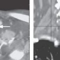
FIGURE 3.3. Examples of three-dimensional (3D) gradient echo techniques. A: A steady state sequence producing a series of contiguous common nominally 1-mm thick sections through the posterior fossa showing the exquisite detail of the very gracile of the cranial nerve VI (arrows) as it courses through the prepontine cistern to enter the tiny Dorello’s canal (arrowhead). B: A three-dimensional gradient echo relatively T1-weighted sequence named MPRAGE following contrast enhancement. This sequence produced approximately 0.65-mm contiguous sections through the region of the cavernous sinus and suprasellar cistern demonstrating an optic glioma extending from the intracranial segment of the right optic nerve (arrow) to involve the left optic nerve (arrowhead). (NOTE: The point of this illustration is to emphasize that 3D techniques, if applied to a particular diagnostic problem in a confined area of interest, can produce extraordinarily detailed thin section imaging with magnetic resonance. The main limitation of these 3D acquisitions is their sensitivity to motion and resulting artifacts and image quality degradation.)
High-resolution, thin section, pulse sequences are often required for areas such as the cavernous sinus, sella, orbit, skull base, IAC/CPA, and craniocervical junction. The trade-off between image contrast, spatial resolution, and SNR to produce a certain resolving power for a given object in this region is described in an article by Enzman and O’Donohue4 concerning optimized techniques for detecting intracanalicular acoustic schwannomas. The type of planning described in the article and the foregoing paragraph are essential for developing MRI protocols for specific indications in each head and neck region. A close look at image contrast issues in the next section reveals that both T1W and T2W images are required in almost all clinical situations. The following discussion concentrates on how to optimize the high-resolution, thin section images routinely required in head and neck imaging and the techniques used to produce them. Always assume that SNR per voxel will be even more critically affected when conventional and, to a lesser extent, fast T2W pulse sequences are necessary.
Slice Thickness
The shape of the slice-selective RF pulse used with 2DFT techniques creates an interesting problem when trying to do contiguous thin (3- to 5-mm) sections. The RF pulse possesses a curved profile; thus, if the scanned sections lie too close together, their edges will overlap in a multislice acquisition (Fig. 3.4). This is usually called cross talk and is most noticeable in long TR/TE acquisitions. The partial saturation of signals that occurs because of this overlap is undesirable in a situation in which much of the SNR per voxel is inherently low because of the thin sections and a relatively small FOV used. Solutions to this vary with different manufacturers. Some approaches perform the multislice acquisition in an interleaving or concatenating pattern (i.e., in the acquisition, a full SLT gap is skipped, offset, and with the gaps obtained with a second acquisition). Other approaches leave a small gap stated to be 15% to 20% of the SLT and accept “noncontiguity,” but this really is not an ideal solution when sections ≤5 mm are required. Most manufacturers have developed more square-shaped pulses to minimize cross talk. The 3DFT techniques can produce excellent-quality 1- to 2-mm (or thinner) truly contiguous sections; time constraints dictate that these be used with gradient echo (GE) techniques (Fig. 3.3).

FIGURE 3.4. Line diagrams demonstrating pulse-shaping techniques that are aimed at producing high-resolution thin sections while minimizing signal-to-noise losses. A: Gaussian slice selection in the time domain (left); thus, the slices will be without any intervening gap. However, the gaussian shape of the slice profile (right) shows considerable overlap of the actual sections that results in partial saturation of adjacent tissue in the sections indicated by the shaded areas. Note from the numbers that the slices may be sampled out of order to somewhat decrease the signal-to-noise effect of choosing a gaussian-shaped pulse for contiguous sections. B: The sin C pulses in the time domain (left) produce a more trapezoidal slice profile than seen with the gaussian pulses in (A). The diagram on the ri ght shows a reduction in the area of overlap or cross talk between the sections that would significantly lower signal signal-to to-noise losses. c –C: The slice selection pulses for a three-dimensional Fourier transform spin echo sequence has a repetition time of half or less of a two-dimensional Fourier transform spin echo sequence. Each pulse perturbs a slab of tissue. The individual sections are then selected by a second phase-encoding gradient with the number of steps in the gradient being equal to the number of slices desired within the slab. This technique produces grossly gapless imaging and eliminates cross talk. There is signal-to-noise drop off at each end of the slab selective pulse that would be worse if a gaussian profile were used to select the slab.
The cephalocaudal extent of a study is a critical parameter in MRI protocol design when using thin sections. Standard SE techniques on most MR units have a duty cycle for SE sequences of about 50 milliseconds per section, mainly due to gradient switching times. During the average 500- to 600-millisecond TR utilized for a T1W sequence, about ten sections can be acquired depending on the TE, bandwidth, and whether flow compensation is used. If 2-mm sections with a TR ≤500 milliseconds are desired, this means that only ≤2 cm of anatomy will be covered. If the region of interest is larger than the region covered in one acquisition, then a second acquisition must be done, prolonging the total series scanning time and thus risking the appearance of motion degradation. Rapid sequential GRE techniques are not likely to replace standard SE sequences for studying the head and neck. The idea of a fast, single-slice technique similar to single-slice sequential CT might be appealing; however, the contrast and spatial resolution of these pulse sequences are not sufficient for demonstrating pathology at many sites. Sensitivity to magnetic susceptibility also limits usefulness of GRE sequences due to the many air–bone interfaces in the head and neck. The 2DFT multislice, SE, and 3DFT GE techniques remain the mainstay of head and neck imaging.
Acquisition Matrix
Acquisition matrix size is a more critical issue with MRI than CT because of its direct impact on imaging time. The acquisition matrix size in the readout (frequency-encoding) gradient direction is usually 256; this number can be increased to 512 simply by increasing the computer’s sampling rate without a penalty in imaging time and only a small cost in image processing time, although SNR will decrease accordingly. However, the matrix size in the phase-encoding direction depends on the number of gradient (row acquisition) steps used during the acquisition. The number of phase-encoding gradient steps is directly proportional to imaging time, as represented by the following equation:
Imaging time = TR × Phase-encoding steps × Number of excitations
Because the FOV is square, a 256 × 256 matrix produces square pixels. On the other hand, a 128 × 256 or 192 × 256 matrix image may be obtained in one half or three quarters of the time, respectively, but the pixels will be rectangular in shape. At a 192 × 256 matrix, this does not produce any visually disturbing artifacts, but the use of a 128 × 256 matrix results in a “truncation” artifact, which is observed as parallel bands that are especially noticeable at borders of markedly different signal intensity (e.g., fat–muscle interface) and that “ring through” the image; time savings must be weighed against image quality in this case. A 192 × 256 or 256 × 256 matrix should be used whenever spatial resolution is an overriding concern. Fewer phase-encoding steps may be possible without significant truncation artifacts. A 512 × 512 acquisition matrix is even practical if the number of signal averages required can keep acquisition time clinically reasonable (about ≤4 to 6 minutes). This creates unacceptably noisy images at field strengths under 1 T. An effective 512 × 512 matrix can also be used in a reasonable time frame, with more signal averages if the phase-encoding steps are made only over the portion of the FOV containing the anatomy in question (i.e., not over the air to each side of the head) with rectangular FOV techniques. The time savings are, again, directly proportional to the number of phase-encoding steps that can be eliminated without ignoring the more useful data within the anatomic limits of the structure being studied.
Field of View
The basic trade-offs in SNR caused by decreasing the FOV were discussed in Chapter 1. When the voxel size is reduced in two dimensions, the decrease in SNR is considerable. At field strengths of 1.0 to 1.5 T, an FOV ≤20 to 24 cm down to 10 to 12 cm are possible with adequate SNR results when using standard eight-channel head coils. Less efficient coils—for example, a nonquadrature Helmholtz pair for the neck—can be used in fields ≥1.5 T.
There is another problem in MRI if the FOV is selected too small. If the receiver coil detects signals from anatomy outside the FOV, the reconstruction processes will place those data in the display. This is referred to as an aliasing, “foldover,” or “wraparound” artifact (these are explained further in a following section on artifacts). This can be avoided by choosing a larger FOV or by matching the volume of tissue detected by the receiver coil (sensitive volume) more closely to the FOV chosen; the latter can be accomplished by using smaller, localized receiver coils or sometimes just centering the anatomy better in the existing coil. An additional benefit of the use of a smaller coil is that it can be more closely coupled to the area of interest and thus suffer less signal losses (noise) from body-related loading. The merging of a closely coupled small-volume receiver coil and small FOV are then a logical combination for high-resolution thin section imaging of a relatively small area of interest such as the temporal bone, TMJ, or eye. Such small coils can be of quadrature design and multiplexed in a phased array to provide very high-resolution (small FOV) images over a larger region than one coil could examine efficiently. This latter concept has been most fully exploited in newer multichannel receiver improvements in MR systems since about 2003.
CONTRAST RESOLUTION
No matter how the MRI sampling is done, relaxation times (T1 and T2), proton density, and flow (motion) will always influence tissue contrast. The sampling can be biased by varying TR, TE, and TI (inversion time), but one must understand the clinical reasons for introducing more T1 or more T2 weighting in the images. The reasons vary with the clinical questions at hand, the need for spatial resolution versus image contrast, and the region or anatomy versus pathology under study. With GRE techniques, the flip angle selected may also be varied to affect contrast. GRE images are also flow sensitive and can be used to dramatically alter contrast due to flow effects.
The study of brain pathology is fairly standardized. Most centers use a combination of FSE and/or fast IR T2W sequences and T1W sequences, preferably in the same plane. A paramagnetic contrast agent may be used, depending on the clinical situation. The detection of intra-axial pathology requires a relatively T2W image with sections ≤5 mm. The choice of a specific T2W pulse varies somewhat between systems, but any work well for detecting intra-axial pathology. In the earlier days of MRI, T2- and density-weighted pairs were used. These have yielded completely to FSE and fast IR (inversion spin echo) sequences since the late 1990s.
In the extracranial compartment, there are tissue contrast issues that are far more complex than those involved in demonstrating brain pathology. The general principle that tissue contrast improves with more T2 weighting for the brain does not hold, because pathologic tissue must be differentiated from several types of surrounding tissue and reactive changes. For instance, tumor imaging below the skull base requires pulse sequences that contrast tumor with fat, muscle, and lymphoid tissue; however, highly spatially resolved images (Figs. 21.43 and 29.16) are also necessary for showing detail such as the precise limits of a lesion relative to the skull base.
T2W images usually provide good tumor–muscle contrast and T1W images and provide good tumor–fat contrast (Table 21.1). Neither T1W nor T2W images will provide reliably predictable contrast between tumor and lymphoid tissue (Chapter 21). Normal lymphoid tissue tends to have a characteristic, convoluted gross morphology on gadolinium (Gd)-enhanced studies that can help with this differentiation; however, ultimately such morphologic features are not sufficient to distinguish tumor and normal lymphoid tissue. Gd enhancement will often improve tumor–muscle contrast on T1W images, but this definitely diminishes tumor–fat contrast (Fig. 14.13). One can give Gd in combination with fat-suppressed, contrast-enhanced (FSCE) images to overcome this difficulty, but enhancing tumor may then be difficult to tell from enhancing lymphoid tissue, salivary gland tissue, and the pterygoid venous plexus. Depending of the region of interest, FSCE images may suffer from susceptibility artifacts imposed by frequency selective FS that are discussed subsequently.
Considering the number of variables just described and the frequent need for displaying pathology in more than one plane, one can see the difficulty that arises in trying to develop “simple,” inclusive protocols for MRI. The best approach is to be aware of the trends just mentioned and exploit the added strength of MRI for tissue contrast resolution compared with CT using MRI to answer focused, clinically relevant questions. Basic pathologic issues such as the preferred sequences for separating tumor from scar or obstructive sinus disease are presented in more detail in conjunction with specific pathologies and general patterns of disease in Chapters 7 through 43.
Specific uses of various pulse sequences are discussed in conjunction with specific disease entities and a simplistic view that “one or two pulse sequences fits all” should never be adopted. Each pulse sequence should be thought out for each particular diagnostic problem in each anatomic region of interest. Such efforts at proper protocol development will be rewarded (Appendix B).
FAT SUPPRESSION AND CHEMICAL SHIFT ARTIFACT
An artifact encountered particularly in orbital MRI is chemical shift or water–fat shift (WFS). The source of this artifact is a difference in shielding by the electrons surrounding hydrogen in water and fat. This results in a difference in resonance frequency between water and fat. While frequency encoding is applied during acquisition, a difference in frequency is interpreted as a different point of origin of the signal during reconstruction of the image. WFS occurs when the water component of the image is shifted with regard to the fat image. As can be understood from its origin, WFS is seen along the frequency-encoding direction (Fig. 3.2). In images, fat can either move away from or move over adjacent tissue, depending on the direction of the applied gradients. This causes either a dark or a bright band at fat–water interfaces. The artifact increases at higher field strength. The WFS decreases with broader receiver bandwidth at the expense of SNR. Although WFS will still be present, FS techniques will render the WFS artifact invisible.
The bright signal from fat on T1W, proton density–weighted, and FSE images creates three main challenges. First, this bright signal truncates the dynamic range of the imaging (scaling), sometimes making optimal visualization of pathology difficult at one window setting. This is less problematic with workstation compared to film-based interpretation. Second, the bright signal from fat reduces contrast between pathologic processes that enhance with paramagnetic contrast agents and fat within tissue and marrow spaces. Third, bright fat signal often diminishes extracranial tumor-to-fat contrast on non-FS FSE images. A frequency-selective FS technique overcomes these problems. Short T1 inversion recovery (STIR) is not considered an FS technique for the purposes of this discussion. STIR, in reality, is a fat-nulling technique that also eliminates the signal from areas of Gd enhancement. STIR has other limitations, including relatively long acquisition time, bounce-back artifact, and sensitivity to flip angle errors. Also, it is difficult to obtain thin, contiguous sections because signal averaging is limited due to the long TR that extends acquisition time. The technique is also sensitive to partial saturation of adjacent slices so that interslice gaps must be utilized, frequently on the order of 50% of the SLT. FSE versions of STIR sequences also null the signal from paramagnetic contrast agents and have other limitations, making them unsuitable for routine use.
FSFS and STIR work well in the orbit and are most valuable when evaluating the optic nerve. Other FS techniques for imaging have given way to frequency-selective FS. The advantages of FS are clear:
(1) Improves contrast between fat and lesions enhancing with Gd (Figs. 21.37, 21.42, and 26.4)
(2) Eliminates chemical shift artifact
(3) Improves dynamic range on FSE T2W images, eliminating the problem of diminished tumor-to-fat contrast seen with this approach to T2 acquisition
(5) Allows the specific diagnosis of a lesion containing mature fat
(5) Is useful in detecting pathology in fat-containing areas such as the mandible and marrow spaces of the skull base (Fig. 21.42)
Artifacts and technical limitations are common with FS techniques. These are often unpredictable in the central and posterior skull base, along the orbital floor, in the oral cavity, and at the thoracic inlet, to name a few common areas. Because of these limitations, protocols that rely strictly on FS T1W images as the only postcontrast T1W acquisition may not contain very important diagnostic information. More specifically, the most important problems that affect protocol development and diagnostic accuracy include the following:
(1) The FS acquisitions have an increased sensitivity to magnetic susceptibility effects that can severely limit scan quality near the paranasal sinuses, aerated temporal bone, and oral cavity as well as in the vicinity of any strongly paramagnetic implanted substance or device (Figs. 1.3 and 1.4). This effect is even more problematic at 3 T (Fig. 1.4).
(2) Inhomogeneity of FS occurs frequently. This is highly dependent on the FOV, positioning of the area of interest in the receiver coil, the receiver coil design, and the overall homogeneity of the main magnetic field as well as that in the specific area of interest. For instance, it is a particular problem at the shoulder–neck junction in larger part due to coil-loading issues (Fig. 3.1). To some extent, this can be overcome with a combination of newer chemical shift FS techniques, but these require relatively long acquisitions. This can be mitigated by combination with newer fast imaging sequences, which may produce some relief from this problem at the shoulder–neck junction, where it is particularly troublesome.
(3) There may be difficulty distinguishing between enhancing pathology and lymphoid tissue, venous plexuses, and some salivary glands on fat-suppressed T1W images and possibly similar problems with contrast on T2W images (Table 21.1).
FS techniques can be combined with 3DFT. It would be appealing to combine a fast acquisition with an FS technique suitable for use with intravenous (IV) paramagnetic contrast agents. Presently, most “fast” T1W imaging requires a GE pulse sequence; these will tend to aggravate the susceptibility artifacts already degrading the fat-suppressed images of the extracranial head and neck.
Paramagnetic Contrast
Gd-DTPA was the first U.S. Food and Drug Administration–cleared contrast agent developed for use with MRI. The mechanism of enhancement with this agent is explained in a later section on magnetic susceptibility and paramagnetic effects. Several other compounds have been developed and are available. This family of compounds depends on the presence of a strongly paramagnetic element (e.g., Gd) that can form a stable chelate. It is injected in very small concentrations (e.g., 0.05 to 0.30 mmol per kg) and is generally safe. Informed consent must be documented when used during pregnancy. There is more recent data indicating that in certain populations, renal toxicity resulting in nephrogenic fibrosis occurs. This now requires renal screening prior to even the lowest dose usage of Gd containing IV contrast agents.
The contrast, like iodinated compounds, accumulates in areas of blood–brain barrier breakdown or other extracellular spaces. At the doses used, the Gd-containing compound produces a much stronger spin alignment; thus a preferential, dramatic T1 shortening of tissues is observed where it localizes. Actual contrast ratios will depend on (a) the relative concentrations of Gd in the lesion versus those in the surrounding normal tissues; (b) the time course of its accumulation and clearance from the normal and pathologic compartments; and (c) the inherent contrast in these areas, which is dependent on the T1, T2, and proton density of the tissue versus pathology and also on the pulse sequence(s) selected for study. Field strength does not seem to be a significant issue even though this is a T1-based phenomenon.
Since Gd enhancement is only effective with T1W pulse sequences, standard 2DFT T1W SE sequences are used most frequently so that high-resolution scans are relatively easy to perform. Both 2DFT and 3DFT GRE techniques may also be used. FS T1W SE sequences are particularly advantageous when enhancing pathology and must be contrasted with surrounding fat (Figs. 21.34 and 21.37). There is some T1 weighting in fast IR, predominantly T2W images, so that needs to be taken into account when such images are incorporated into protocols using Gd injection as part of the examination. STIR sequences are not effective when used in conjunction with Gd because its signal, which arises from enhanced areas, is nulled along with the fat since they have a similar T1 relaxation time.5 Some contrast enhancement may be seen on the T2W fast IR sequences, but no significant effects are visible on heavily T2W images. When used with fast, flow-sensitive techniques, these contrast agents can improve visualization of smaller vessels and those with slower flow rates. Dynamic studies with Gd enhancement have also been used to study regional brain perfusion and flow dynamics in dural venous sinuses, the pituitary gland, brain tumors, and various vasoformative lesions. It is used experimentally for perfusion imaging of lymph node metastases and primary tumors; however, this is not recommended as a clinical routine at this time (Fig. 21.63).
Intracranially, contrast is useful for detecting intra- and extra-axial pathology. Intra-axial disease is demonstrated because of its inherent vascularity and/or blood–brain barrier breakdown. Extra-axial disease processes requiring Gd enhancement include masses such as meningioma, those arising from or spread along cranial nerves, and meninges. There is no question that the use of paramagnetic contrast agents improves the detection and evaluation of the extent of intracranial disease; this must be tempered by knowledge of how normal structures in a particular area of interest might enhance. Newer Gd agents actually increase the likelihood of seeing normal structures such as the dura enhance, and this must be taken into account if such a transition to newer agents occurs in a particular practice setting.
The value and role of Gd enhancement in the evaluation of extracranial head and neck pathology varies more than that just described for intracranial lesions. The meningeal and cranial nerve pathologies just emphasized stand at the interface of intracranial and extracranial disease and require contrast for complete evaluation. IV contrast can also be useful in differentiating inflammatory sinus disease from masses. It can help better define the extent of some masses and improve lesion–muscle contrast (Figs. 21.18 and 21.40). However, it can significantly decrease lesion–fat contrast and potentially mask the margins of pathology at fatty interfaces (Table 21.1). This is particularly disturbing at the skull base, where evidence of a pathologic process extending into the fatty marrow can completely disappear following contrast injection (Fig. 14.13A–C). This can be overcome to some extent by using fat-suppressed T1W images in conjunction with Gd enhancement.6 However, on fat-suppressed, Gd-enhanced images, enhancing pathology may become isointense to the enhancing pterygoid and other venous plexuses just below the skull base (Table 21.1). The uses of paramagnetic contrast in general pathologic terms are discussed in conjunction with general theories of MR image acquisition earlier in this chapter and its use in specific clinical situations in the remaining chapters.
RELAXATION PROCESSES: T1, T2, AND THE EFFECTS OF PARAMAGNETIC SUBSTANCES AND SUSCEPTIBILITY
The concept of relaxation is as fundamental to understanding MRI as the concept of the voxel (Chapter 1) is to both CT and MRI. In fact, if one simply has a working knowledge of the voxel and that of relaxation processes, much of the complexity of MR interpretation is diminished. Although proton density and flow also influence image contrast, the relaxation processes have a dominant effect on how the images appear with regard to selection of pulse sequence parameters for a specific diagnostic purpose. Once understood, the concepts presented in this section will provide a framework for understanding findings on MR images that are sometimes perplexing, such as changes in signal during clot evolution, why secretions in sinuses may have such a diverse appearance, and how to anticipate when certain pulse sequences will be unsuccessful because of poor tissue contrast and/or increased sensitivity to artifacts.
Since this chapter emphasizes concepts of both basic and applied physics, the reader may want to consult other, more technical references on topics such as nuclear spin and relaxation processes.7,8 In particular, it would be useful to understand the basics of nuclear spin behavior in the presence of static magnetic and RF fields, T1 relaxation and T2 decay curves, and the quantum mechanical (thermal equilibrium) and rotating frame models of relaxation.
This section deals with the causes of spin relaxation—that is, the origins of T1 and T2—and then goes on to describe how these phenomena relate to paramagnetic and magnetic susceptibility effects. The discussion draws heavily on the notes of lectures given by Professor E. Raymond Andrew to practicing radiologists and trainees at the University of Florida. We are forever indebted to Professor Andrew for his clarity of thought, insights, skillful teaching, and kindness.
In order to understand the basic concepts of the spin-lattice and spin-spin relaxation processes, it is first necessary to re-emphasize the fact that when the nuclear spins are immersed in the external static magnetic field, they reach a steady state of thermal equilibrium, in which the majority of the spins is in a lower energy state—that is, aligned with the magnetic field. However, the laws of quantum and statistical physics indicate that some of these spins will be in a higher energy state, aligned against the field. The difference between the energies of these two states is discrete (i.e., only one energy, not a spread of energies), predictable, and well known. The state of thermal equilibrium is disturbed by the application of an RF pulse of a very specific energy and therefore of a very specific, single, resonant frequency, with resonant meaning “of the same frequency.” H protons in the lower energy level are provided by the RF pulse with the exact amount of energy needed to jump to the higher energy level. Slightly higher or slightly lower energies will not result in the absorption of energy by nuclear spins, as they can only be in either the lower or the higher energy state and nowhere else. The longer the RF pulse remains applied to the sample, the larger the number of nuclear spins transitioning or jumping from the lower to the higher energy state. This can be related to the known fact that the macroscopic magnetization changes direction depending on the saturation of the RF pulse controlled by the so-called “flip angle.” As the RF pulse is turned off, nuclear spins will begin transitioning back to the lower energy state, returning to the “natural” state of thermal equilibrium. In doing so, they release the energy that they absorbed initially from the RF pulse. This energy cannot be of any other frequency but the resonant frequency, as the nuclei must release exactly that much energy to “land” on the lower energy state, since no other energy state is possible. The process of returning to the lower energy state while releasing energy is called relaxation, and the times required for nuclear spins to return to their lower, thermal equilibrium states are called relaxation times. These relaxation times are tissue and substance specific.
Importance of the Total Local Magnetic Field and Molecular Motion
The relaxation of nuclear spins back to their steady state of thermal equilibrium, which results from being under the influence of the static magnetic field only, is fundamentally influenced by the local inter- and intramolecular magnetic fields and the precessional frequency of the molecules to which the nuclei (hydrogen protons) are attached. Of these two, local magnetic fields have a definitive impact on the relaxation processes. In tissues, every H proton has at least one other H proton in the vicinity of a water molecule. In a water molecule, the hydrogen protons are only 2 × 10⁻¹⁰ m away. They each generate and exert a local magnetic field of about 5 gauss on each other. In more complex molecules such as proteins, lipids, and carbohydrates found in all tissues, every H proton has one or two H protons in its vicinity. Thus, it becomes apparent how all protons experience a local internal magnetic field that is referred to as local field intensity in accompanying illustrations (Fig. 3.5) on the order of a few gauss. The intensity and direction of the total local magnetic field experienced by each H proton local field fluctuates because the water molecules are turning and moving around in an average time of approximately every 10-11 seconds (correlation time) at 37?C. This thermal or “Brownian” motion causes molecules to move randomly rather than uniformly as they precess, thus buffeting all other molecules in the solution. The random motion produces a spread of precessional frequencies of up to 10-11 Hz, which is the reciprocal of the correlation time of 10-11 seconds (Fig. 3.5). The combined “tumbling” motion of all spins in a sample occurring with these frequencies drives the energy exchange between the sample as a whole (also called the lattice) and the individual spins that result in their relaxation to thermal equilibrium. The motion of the molecules just described allows for the dissipation of the excess energy and a return to thermal equilibrium, or so-called spin-lattice relaxation. This process takes place at a specific rate, represented by a characteristic time T1 (the spin-lattice relaxation time).

FIGURE 3.5. A series of graphs demonstrating the principles of relativity as described in detail in the text. A: Local field intensity plotted against the distribution of motional frequencies demonstrating the behavior of pure water. B: The same axial and ordinate factors demonstrating the differences in behavior of tissue and pure water that account for differences of observed T1 and T2 effects in magnetic resonance images. C: The same plot as in (A) and (B) showing the effects of paramagnetic contrast on T1 relaxation relative to T2. One can see that the effects are relatively independent of field strength and the effects are far more on T1 than T2 relaxation but that there is a measurable if not visible T2 effect.
Related posts:
 Fibrous Dysplasia and other Fibro-osseous Lesions of the Craniofacial Skeleton
 Intraconal Orbit: Tumors
 Hypopharynx: Developmental Abnormalities
 Tumors of the Submandibular Gland and Space and Tumorlike Conditions
 Masticator Space, Buccal Space, and Infratemporal Fossa Infections and Other Inflammatory Conditions
 Oral Cavity and Floor of the Mouth: Malignant Tumors
Stay updated, free articles. Join our Telegram channel

Full access? Get Clinical Tree


