A. Magnetic nuclei
–Magnetic resonance (MR) relates to interactions with nuclei.
–Because of their nuclear charge distribution, some nuclei have nuclear magnetization.
–Magnetic nuclei can be represented by a vector that depicts the strength and orientation of the nuclear magnetization.
–Nuclear magnetization may be called magnetic dipole, magnetic spins, or magnetic moments.
–Nuclei with an even number of protons and an even number of neutrons have no nuclear magnetization.
–Even numbers of protons pair up with their magnetization aligned in opposite directions and cancel each other (as do even numbers of neutrons).
–Nuclei with an odd number of protons, or odd number of neutrons, have a nuclear magnetization.
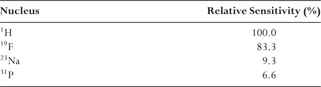
–These magnetic nuclei can be considered to behave like bar magnets and are candidates for magnetic resonance (see Table 11.1).
–Hydrogen nuclei have the largest nuclear magnetization.
–The abundance of hydrogen in the body, together with the large nuclear magnetization, makes it the basis of most clinical magnetic resonance (MR) imaging.
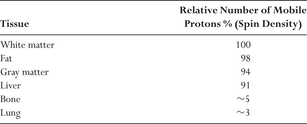
–Detected MR signals originate in protons in free water (i.e., mobile) and fat.
B. Tissue magnetization
–There are more than 1022 hydrogen protons in each cubic centimeter (cm3) of tissue.
–Protons are normally randomly oriented and, have no net nuclear magnetization.
–When placed into a magnetic field, hydrogen nuclei (protons) will become orientated either spin up (i.e., aligned along the field) or spin down (i.e., aligned opposite to the field).
–Spin-down alignment corresponds to a slightly higher energy level.
–A small excess of protons go into the spin-up alignment.
–This excess is ~4 for each million protons at 1 tesla.
–Magnetic fields of the remaining spin-up and spin-down nuclei cancel.
–Tissue placed into a magnetic field produces a net nuclear magnetization of unpaired protons aligned in the direction of the external field.
–Only these excess nuclei in the lower energy (spin up) state contribute to the MR signal.
–One reason that MR signals are weak is that so few nuclei contribute to the MR signal.
–Considerable technical ingenuity is required to maximize the MR signal-to-noise ratio (SNR).
–Table 11.2 summarizes the relative amounts of mobile protons in different tissues.
C. Larmor frequency
–When magnetic nuclei are placed into a magnetic field, a torque causes the moments to perform a precession motion similar to a spinning top.
–The Larmor frequency (fL) is the precession frequency (MHz) of nuclei in a magnetic field (Bo).
TABLE 11.1 Nuclei Used in MR and Their Relative Sensitivity
–The Larmor frequency is directly proportional to the magnetic field strength.
–Larmor frequency (fL) for protons is 42 MHz at 1 T.
–The Larmor frequency for protons is 21 MHz at 0.5 T and 127 MHz at 3 T.
–These frequencies are in the ham radio and aviation radiofrequency range.
–19F has a Larmor frequency of 40 MHz at 1 T.
–23Na has a Larmor frequency of 11 MHz at 1 T.
–For nuclei of interest in clinical MR, protons have the highest Larmor frequency at any field strength.
–Increasing the Larmor frequency results in higher MR signals.
D. Resonance
–Radiofrequency (RF) electromagnetic fields are generated using a volume or surface coil.
–Resonance occurs when an applied RF field interacts with the net nuclear magnetization.
–The applied RF must be at the Larmor frequency, and its orientation must be perpendicular to the external magnetic field.
–RF at frequency fL, when applied perpendicular to the external magnetic field, causes the magnetization vector to rotate.
–The rotation of the magnetization continues while the RF is being applied (i.e., is switched on).
–When the RF is switched off, the magnetization will have rotated through an angle called the flip angle.
–The flip angle depends on applied RF field strength and the total time that it is on (i.e., pulse duration).
–A 90-degree RF pulse reorients the magnetization vector to a direction 90 degrees perpendicular to the direction it had prior to the pulse.
–A 180-degree RF pulse reorients the magnetization vector to a direction 180 degrees (i.e., opposite) to the direction it had prior to the pulse.
–A 90-degree RF pulse takes half as long as a 180-degree RF pulse.
–The component of the net magnetization vector parallel to the main magnetic field is called the longitudinal magnetization.
–By convention, the longitudinal magnetization is taken to point in the z-axis.
–The component perpendicular to the main magnetic field is called the transverse magnetization.
–By convention, the transverse magnetization is taken to be in the x-y plane.
TABLE 11.2 Relative Amounts of Mobile Protons in Different Tissues
–After a 90-degree RF pulse is applied to longitudinal magnetization, the resulting transverse magnetization vector precesses about the external magnetic field.
–The precession frequency is also the Larmor frequency fL.
–This rotating magnetization can be detected as an induced voltage in a coil.
–An RF coil is simply an optimized antenna, and the detected signal will be stronger the closer the coil is to the signal source.
–The detected voltage is called the free induction decay (FID) signal.
–The FID signal is an oscillating voltage at the Larmor frequency (fL).
–The induced FID is obtained in a receiver coil placed around the sample.
–The FID signal is weak because of the small number of nuclei that contribute to the signal (i.e., ~4 per 106).
–Nuclear magnetization is ~700 times weaker than electron magnetization.
–The small size of all nuclear magnetic moments results in a weak FID signal.
–Receiver coils may be the same as transmitter coils.
–FID signals are detected, digitized, and used to produce MR images.
A. T1 relaxation
–Protons placed into magnetic fields produce a net magnetization with a magnitude Mz (i.e., longitudinal magnetization).
–Mz is parallel to the direction of the external magnetic field.
–Longitudinal magnetization grows exponentially from the initial value of zero to the equilibrium value of Mz with a time constant T1 (Fig. 11.1).
–At a time equal to T1, 63% of the magnetization has formed.
–Full magnetization (i.e., Mz) is normally taken to occur after a time interval of approximately 4 × T1.
–If the external magnetic field is switched off, longitudinal magnetization Mz decreases exponentially with the same time constant T1.
–Longitudinal magnetization decays as Mz× e−t/T1 where t is the elapsed time.
–T1 relaxation is called longitudinal relaxation and spin-lattice relaxation.
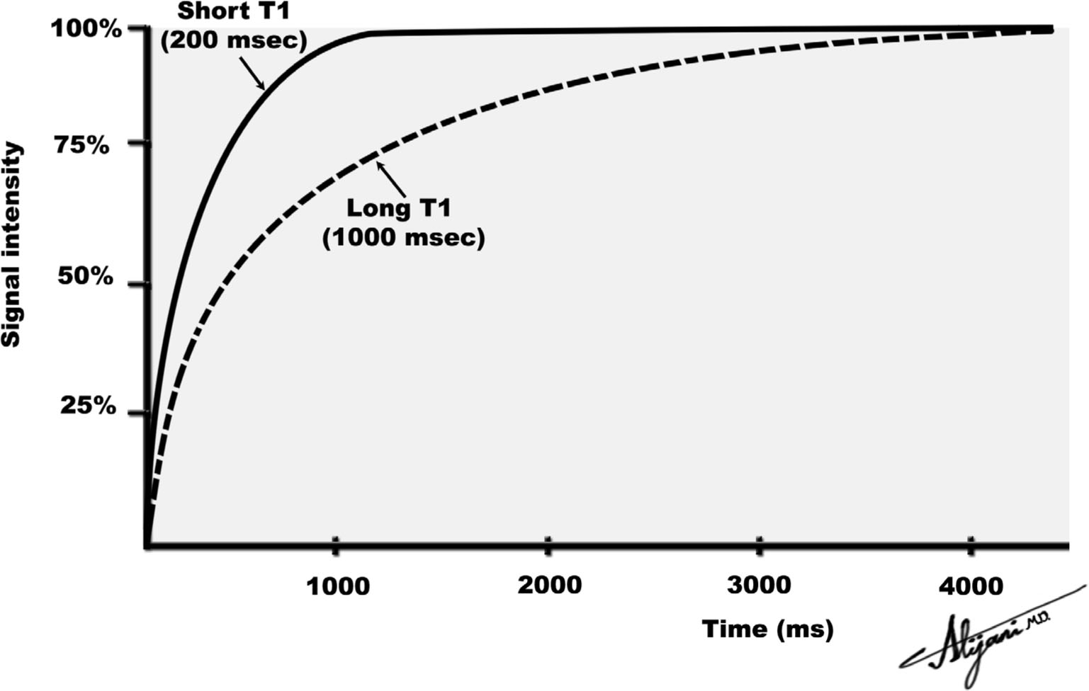
FIGURE 11.1 Return to equilibrium of longitudinal magnetization for two tissues with different T1 relaxation times.
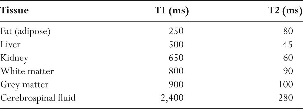
TABLE 11.3 Representative T1 and T2 Relaxation Times (1.5 Tesla)
–When the lattice has components of motion at the Larmor frequency, this “encourages” a nucleus to interact with the surrounding jiggling spins and undergo recovery.
–Different tissues have different frequencies of motion (vibration modes), which accounts for the differences in T1 relaxation times.
–T1 is long in liquid materials (cerebrospinal fluid [CSF]) and in solids (hair).
–T1 is short in medium-viscosity materials and in fat (Table 11.3).
–Contrast agents such as gadolinium-DTPA cause T1 to be shortened.
–For tissues, T1 increases with increasing magnetic field strength.
–Doubling the magnetic field strength increases tissue T1 by approximately 20.5.
B. T1 contrast
–Generating a N2 matrix MR image requires the acquisition of N sequential signal acquisitions that are obtained with a repetition time TR.
–In time TR, one signal (i.e., one line of data) is obtained, which contains 256 values.
–In the second TR interval, another line of data is acquired, and so on.
–The value of TR is entirely under the control of the operator and ranges from tens of milliseconds to seconds.
–The choice of TR value affects the contrast between tissues that differ in their T1 values.
–A long TR value permits the magnetization in all tissues to fully recover.
–As a result, long TR times generate no T1 weighting.
–When TR values are short, only tissues with short T1 values fully recover their longitudinal magnetization and contribute a signal.
–With short TR values, tissues with a long T1 do not recover and therefore contribute little signal.
–A T1-weighted image is obtained using short TR that emphasizes T1 differences.
–Short TR times are less than ~300 ms at 1.5 T and less than ~450 ms at 3T.
C. T2 relaxation
–After a 90-degree pulse, the magnetization vector rotates at the Larmor frequency in the transverse (x-y) plane.
–The FID signal produced is proportional to the x-y magnetization vector.
–In perfectly uniform magnetic fields, the transverse magnetization decays exponentially with a time constant T2 (Fig. 11.2).
–The induced FID signal decays as e−t/T2 where t is the time.
–At a time equal to T2, the signal has decayed to 37% of its original value.
–After a time ~4 T2, the transverse magnetization signal is negligible.
–T2 relaxation is called transverse relaxation.
–T2 relaxation is also known as spin-spin relaxation as it is mediated by interactions between the magnetic fields of adjacent nuclei (spins).
–For most tissues, T2 times are tens of milliseconds (Table 11.3).
–Liquids have long T2 times whereas viscous materials and solids have short T2 times.
–T2 decreases with increasing viscosity and decreasing molecular mobility.
–Tissue T2 values are approximately independent of magnetic field strength.
D. T2 contrast
–MR signals are most often obtained in the form of echoes from transverse magnetization.
–MR echoes occur at a time TE (time to echo) that is under operator control, and can be selected to be long or short.
–Short TE values will result in little loss of transverse magnetization (i.e., little T2 decay).
–Short TE values therefore produce no differences (contrast) between tissues that have different T2 values.
–Short TE values have minimal T2 weighting.
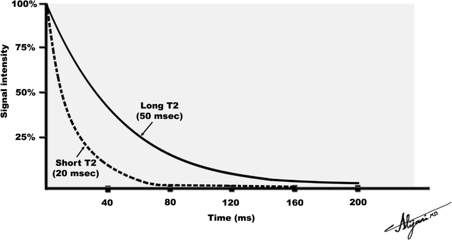
FIGURE 11.2 Loss of transverse magnetization due to T2 relaxation.
–Long TE values will reduce the intensity of transverse magnetization for tissues with short T2 much more than tissues with long T2.
–T2-weighted images are obtained with a long TE.
–Long TE values are typically greater than 60 ms.
E. T2*
–Normal magnets have magnetic field inhomogeneities with slight differences in magnetic field at different locations.
–Magnet inhomogeneities are typically a few parts per million (ppm).
–Magnet inhomogeneities are a few μT in fields of 1 T.
–Inhomogeneities also arise because of different magnetic properties of different tissues (e.g., iron in the blood) and at tissue boundaries (i.e., susceptibility inhomogeneities).
–Differences in magnetic field strength cause magnetization at different locations to rotate at slightly different Larmor frequencies.
–Larmor frequency is proportional to magnetic field strength.
–Adjacent magnetizations that initially point in the same direction start to diverge and point in different directions (i.e., dephase).
–This divergence (dephasing) results in a loss of transverse magnetization.
–Spin dephasing due to inhomogeneities is T2inhomogeneity.
–Decay of transverse magnetization (FID) occurs because of inhomogeneities in the main magnetic field and T2 decay, which is called T2* .
–The observed FID signal falls exponentially with a decay rate constant T2* (i.e., e−t/T2* ).
–The relationship between T2, T2*, and spin dephasing due to inhomogeneities (T2inhomogeneity), is given by 1/T2* = 1/T2 + 1/T2inhomogeneity
–T2* is a few milliseconds and is always shorter than T2.
–For tissues, T2*≤ T2 ≤ T1.
–In soft tissues, inhomogeneities are the most important contribution to T2* .
–Materials such as paramagnetic and ferromagnetic contrast agents disrupt the local magnetic field homogeneity and shorten T2*.
–Dephasing due to the inhomogeneity contribution to T2* may be overcome by generating spin echoes.
–By contrast, loss of transverse magnetization due to T2 relaxation is irreversible.
A. Magnets
–Powerful magnets capable of generating strong magnetic fields are essential for MR.
–MR magnetic fields also need to be stable and uniform in space.
–Magnetic fields are measured in tesla (T).
–1 T = 10,000 gauss (G).
–The earth’s magnetic field is weak (50 μT or 0.5 G).
–To perform MR, the magnetic field must have a homogeneity of only a few parts per million.
–Magnetic shimming is used to make small corrective changes to the main field to improve the magnetic field uniformity.
–Magnetic shimming can be accomplished with passive techniques (pieces of iron at specific locations).
–Active magnetic shimming uses electrically energized coils.
–The large whole-body magnets used in MR scanners may be resistive, permanent, or superconducting.
–Permanent magnets have low operating costs and small fringe fields.
–Limitations of whole body permanent magnets are that they are heavy and generate fields only up to ~0.35 T.
–Resistive magnets can generate magnetic fields up to ~0.5 T.
–Resistive magnets can be turned on and off, but consume a large amount of power and need cooling because of the heat generated.
B. Superconducting magnets
–Current MR uses field strengths higher than those of resistive and permanent magnets.
–Superconductivity is the ability of certain materials to conduct electrical current without any resistance.
–Superconducting MR magnets use a wire-wrapped cylinder (i.e., a solenoid) to generate the uniform magnetic field.
–Superconducting magnets must be kept very cold using liquid helium (4° K) as a refrigerant.
–A perpetually circulating electric current of hundreds of amps creates the magnetic field.
–The superconducting magnetic field is always on.
–If the wire temperature rises, the system loses its superconducting properties and the energy stored in the magnetic field is converted to heat resulting in a magnet quench.
–Figure 11.3 is a cutaway view of a superconducting MR imaging system.
–Field strengths of 20 T can currently be generated by superconducting magnets.
–As MR field strength increases, so does T1 relaxation time, SNR, and RF energy deposition in the patient.
–Some image artifacts may also increase with increasing magnetic field strength.
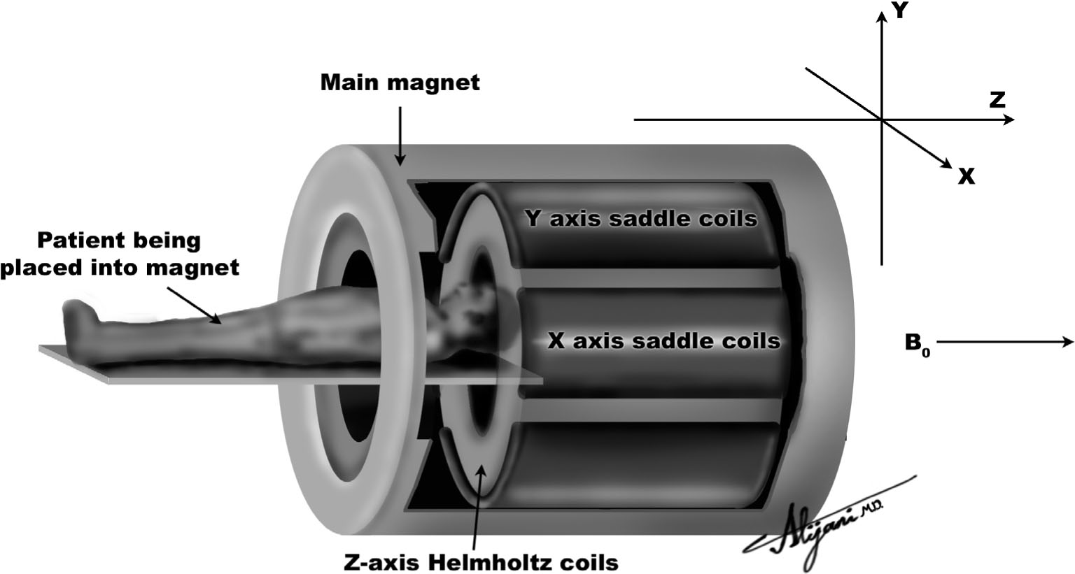
FIGURE 11.3 Superconducting magnetic resonance system showing the main magnetic field (Bo) and three sets of coils that generate magnetic field gradients.
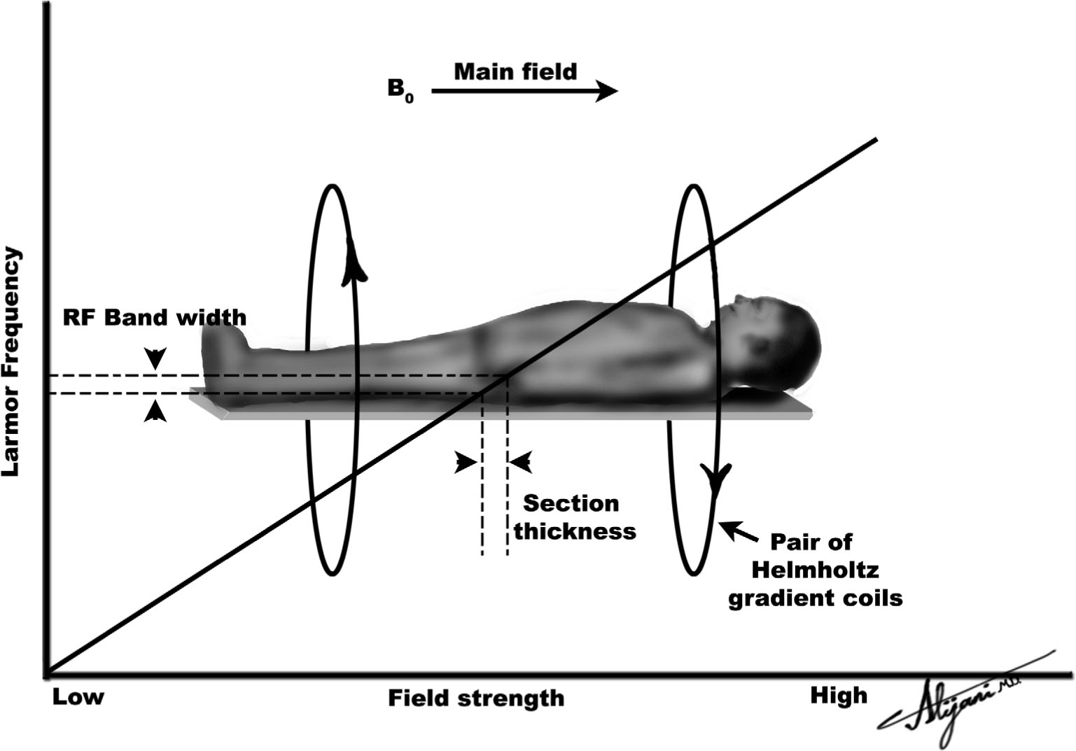
FIGURE 11.4 The solid line shows how the Larmor frequency varies along the long patient axis when a gradient is applied. When an RF pulse with a narrow range of frequencies is used, it only affects magnetization within a narrow distance along the patient, defining image slice thickness.
C. Gradient coils
–Magnetic gradients are used to code the spatial location of the MR signal.
–Gradients are essential for generating images.
–MR systems have three magnetic field gradient coils oriented in the x, y, and z directions.
–Combinations of three orthogonal sets of gradients allow the gradient field to be oriented in any direction.
–Axial gradients (z) are produced using Helmholtz coils.
–Figure 11.4 shows a pair of Helmholtz coils being used to produce a gradient along the z-axis.
–Gradients that change the main field as a function of x or y distance are normally produced by saddle coils.
–When activated, these gradients superimpose a linear gradient on the main magnetic field.
–With gradients superimposed on the main magnetic field, each magnetic field location corresponds to a slightly different Larmor frequency.
–Magnetic gradients cause different locations to have different magnetization precession frequencies.
–Gradient strengths are ~30 mT/m on a 1.5-T scanner.
–Gradients may need to be switched on and off rapidly (<500 μs).
–Gradients generate small, rapidly decaying eddy currents in other coils or metal structures nearby.
–Induced eddy currents impair scanner performance and may create image artifacts.
D. Radiofrequency coils
–RF is electromagnetic radiation with frequencies in the range of approximately 1 MHz to 10 GHz.
–A RF coil consists of various configurations of radiowave antenna.
–Transmitter coils are used to send in RF pulses with the required flip angle.
–Radio waves from transverse magnetization in patients are detected by receive RF coils.
–Receive coils may be physically separate from the transmit RF coil, or may be the same coil switched electronically from transmit mode to receive mode.
–Placing the receive coils close to the region being imaged improves the detected radiowave signal (i.e., increases SNR ).
–Smaller coils generally have lower levels of noise (i.e., will increase SNR).
–Volume coils are designed to transmit and receive uniform RF signal throughout a volume, e.g., the head coil or body coil.
–Specialized RF coils include those for the knee and spine.
–Linear volume coils receive the signal from only one of the x-or y-axes of the rotating transverse magnetization.
–Quadrature volume coils receive the signal in both the x-and y-axes, therefore increasing the overall SNR and reducing image artifacts.
–Surface coils have increased sensitivity close to the coil, but the signal drops off with increasing distance from the coil.
–Phased array coils are a combination of many surface coils around the body part being examined.
–Phased arrays try to obtain uniform signals from the enclosed volume with an improved signal detection of individual surface coils.
–Phased array coils are required for parallel imaging.
E. Parallel imaging
–Parallel imaging uses the separate signals from phased array coils.
–Many individual surface coils in a phased array coil detect the same signal from the same place in the body.
–However, the strength of the detected signal is different in each coil because it is at a different distance from the RF source.
–Using a preacquired sensitivity map of each coil, additional information is obtained from several surface coils.
–Surface coils in a phased array coil used for parallel imaging are termed elements.
–Phased array coils are available with up to 32 elements, with each element having a separate RF preamplifier.
–The parallel imaging factor quantifies the speed-up factor.
–The maximum parallel imaging factor is related to the number of elements.
–High parallel imaging factors produce unacceptable artifacts.
–Parallel imaging factors achieved in clinical imaging range between 2 and 4.
–Parallel imaging works well when high SNR is available, such as from high field 3T scanners.
F. Shielding
–The magnetic flux lines
Related posts:


Stay updated, free articles. Join our Telegram channel

Full access? Get Clinical Tree


