(e.g. a time series of N images with D pixels each) lies on a manifold  which can be described by much fewer dimensions. Manifold learning techniques map each point
  in the high-dimensional dataset to a low-dimensional point
  , where
  , while preserving the local neighbourhood structure of the high-dimensional points on
  . The low-dimensional points form a new low-dimensional dataset
  .
.
LLE models the locality of the high-dimensional space by first constructing a graph of the data points and then calculating the weights which reconstruct each high-dimensional point as a linear combination of its k-nearest neighbours. The optimal contribution of each point j to the reconstruction of i is given by the weights  and can be calculated as described in [11]. The embedding preserving this structure is given by the Y minimising the cost function
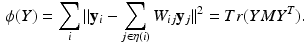
Here,  is the neighbourhood of each point i and
  is the trace operator. This optimisation problem can be solved by calculating the eigendecomposition of the centred reconstruction weight matrix
 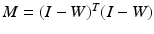 . The embedding Y is given by the eigenvectors corresponding to the second smallest to
  smallest eigenvalues of M [11].
and can be calculated as described in [11]. The embedding preserving this structure is given by the Y minimising the cost function(1)
is the neighbourhood of each point i and is the trace operator. This optimisation problem can be solved by calculating the eigendecomposition of the centred reconstruction weight matrix . The embedding Y is given by the eigenvectors corresponding to the second smallest to smallest eigenvalues of M [11].It is well known that when manifold learning is applied to time series of medical images under free breathing, the low dimensional coordinates  contain useful information about the motion. In particular, when reducing the data to a one dimensional space (
 ) the embedding strongly correlates with a respiratory navigator obtained by traditional means [14]. Baumgartner et al. [1] showed that embeddings in higher dimensions can give additional information on respiratory variation such as hysteresis or respiratory drift over time.
contain useful information about the motion. In particular, when reducing the data to a one dimensional space () the embedding strongly correlates with a respiratory navigator obtained by traditional means [14]. Baumgartner et al. [1] showed that embeddings in higher dimensions can give additional information on respiratory variation such as hysteresis or respiratory drift over time.2.2 Manifold Alignment by Simultaneous Embedding
Medical image datasets which have the same source of motion often lie on similar low-dimensional manifolds. Within the context of this work the different datasets are free breathing images acquired from different views, i.e. different slice positions (MR) or different probe locations (US). Bringing the manifolds into a globally consistent coordinate system allows the matching of images at similar respiratory positions between the different views.
Unfortunately, the embeddings obtained using manifold learning techniques are arbitrary with respect to the sign of the eigenvectors (i.e. arbitrary flipping). In addition, the manifolds obtained from different datasets often feature small but significant differences in shape such as small rotations or scaling differences, which further complicate their alignment. In order to relate the respiratory positions of L different datasets ![$$X_1,\dots , X_L : X_{\ell } = [\mathbf {x^{(\ell )}_1},\dots ,\mathbf {x^{(\ell )}_N} ]$$](/wp-content/uploads/2016/09/A339424_1_En_28_Chapter_IEq15.gif) (e.g. free breathing images obtained from L different views) in the low-dimensional space, first the underlying manifold embeddings
(e.g. free breathing images obtained from L different views) in the low-dimensional space, first the underlying manifold embeddings  must be aligned.
(e.g. free breathing images obtained from L different views) in the low-dimensional space, first the underlying manifold embeddings must be aligned.Our solution to the alignment problem is to formulate a joint cost function and then compute an embedding for all datasets simultaneously in one embedding step. This approach is the general case for L datasets of the formulation proposed in [1] for two datasets. However, to the best of our knowledge, LLE has not been extended to embed ![$$L>2$$” src=”/wp-content/uploads/2016/09/A339424_1_En_28_Chapter_IEq17.gif”></SPAN> datasets simultaneously. This can be done by augmenting the cost function from Eq. (<SPAN class=InternalRef><A href=]() 1) as follows:
1) as follows:
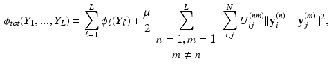
where  is given by Eq. (1). The second term of Eq. (2) is the cost function relating all datasets to each other.
  is a similarity kernel relating points from dataset n to dataset m. Large values in
  force corresponding points to be close together in the resulting embedding.
  is a weighting parameter which governs the influence of the inter-dataset terms.
  can be rewritten in matrix form as
 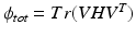 , where V is a
  matrix containing the concatenated embeddings,
 ![$$V = [Y_1,\dots ,Y_L]$$](/wp-content/uploads/2016/09/A339424_1_En_28_Chapter_IEq25.gif) , and
, and
![$$\begin{aligned} H = \left[ \begin{array}{cccc} M^{(1)} + \mu {\sum }_p D^{(1p)} &{} -\mu U^{(12)} &{} \ldots &{} -\mu U^{(1L)} \\ -\mu U^{(21)} &{} M^{(2)} + \mu {\sum }_p D^{(2p)} &{} \ldots &{} -\mu U^{(2L)} \\ \vdots &{} \ &{} \ddots &{} \vdots \\ -\mu U^{(L1)} &{} -\mu U^{(L2)} &{} \ldots &{} M^{(L)} + \mu {\sum }_p D^{(Lp)} \end{array} \right] \end{aligned}$$](/wp-content/uploads/2016/09/A339424_1_En_28_Chapter_Equ3.gif)
Here, the diagonal degree matrices  are given by
  . Under the scaling constraint
  , the embeddings V are given by the second smallest to
  smallest eigenvectors of H.
(2)
is given by Eq. (1). The second term of Eq. (2) is the cost function relating all datasets to each other. is a similarity kernel relating points from dataset n to dataset m. Large values in force corresponding points to be close together in the resulting embedding. is a weighting parameter which governs the influence of the inter-dataset terms. can be rewritten in matrix form as , where V is a matrix containing the concatenated embeddings, , and(3)
are given by . Under the scaling constraint , the embeddings V are given by the second smallest to smallest eigenvectors of H.2.3 Similarity Without Correspondences
All previous work on simultaneous embeddings has either used known prior correspondences to define the similarity kernels  [5], or has used similarity measures between the high-dimensional data to define it [1, 8]. The notable exception is [15] which we discussed in the introduction. For many applications, however, it is desirable to simultaneously embed medical image datasets which are not comparable in image space and for which prior correspondences are not easily obtainable. This problem is effectively one of finding a suitable inter-dataset similarity kernel
  that connects datasets
  but which is not based on comparisons between datasets in the high-dimensional space.
[5], or has used similarity measures between the high-dimensional data to define it [1, 8]. The notable exception is [15] which we discussed in the introduction. For many applications, however, it is desirable to simultaneously embed medical image datasets which are not comparable in image space and for which prior correspondences are not easily obtainable. This problem is effectively one of finding a suitable inter-dataset similarity kernel that connects datasets but which is not based on comparisons between datasets in the high-dimensional space.In this paper we propose a novel, robust method for deriving an inter-dataset similarity kernel. Instead of directly comparing the data from different datasets in the high-dimensional space we first analyse the internal graph structure of each dataset and derive a characteristic feature vector for each node. In the next step we compare these feature vectors across datasets. This approach is an extension of the method proposed in [3] for graph matching.
Deriving a Characteristic Feature Vector for Each Node. For each dataset X we form a fully connected, weighted graph  , connecting each node in V to every other with edges E. The edge weights
  connecting node
  to
to  are given by a Gaussian kernel
 where
where  are the high-dimensional data points of X, and
  is a shape parameter. Note that
  is formed by intra-dataset comparisons only.
, connecting each node in V to every other with edges E. The edge weights connecting node to are given by a Gaussian kernel are the high-dimensional data points of X, and is a shape parameter. Note that is formed by intra-dataset comparisons only.As noted in [3], the steady-state distribution of a (lazy) random walk, i.e. the probability  of ending up at a particular node
  after
after  time steps, can provide information about each node’s location in the graph. In a lazy random walk the walker remains at their current node
  with probability 0.5 at each time step and walks to a random neighbour
  with a probability given by the edge weights
  the other half of the time. The state of the random walk in a weighted graph after
  time steps is given by
  , where B is the diagonal degree matrix given by
  . The steady state distribution is stationary and is given by

In [3],  was used to perform graph matching. In our experiments,
  alone was not sufficiently robust to align our datasets. Therefore, to increase the robustness of this measure we propose to additionally analyse the neighbourhood of each node. For each
  we select the r-nearest neighbours and evaluate their
  as well, by forming an average over the neighbourhood:
 Stable Overlapping Replicator Dynamics for Multimodal Brain Subnetwork Identification
 PET Reconstruction with Sparse Image Representation and Anatomical Priors
 Method to Discover Genetically Driven Image Biomarkers
 Segmentation and Registration Through the Duality of Congealing and Maximum Likelihood Estimate
 Tumor Growth Prediction with Multiplicative Growth and Image-Derived Motion
 Frames for Heart Fiber Reconstruction


of ending up at a particular node after time steps, can provide information about each node’s location in the graph. In a lazy random walk the walker remains at their current node with probability 0.5 at each time step and walks to a random neighbour with a probability given by the edge weights the other half of the time. The state of the random walk in a weighted graph after time steps is given by , where B is the diagonal degree matrix given by . The steady state distribution is stationary and is given by(4)
was used to perform graph matching. In our experiments, alone was not sufficiently robust to align our datasets. Therefore, to increase the robustness of this measure we propose to additionally analyse the neighbourhood of each node. For each we select the r-nearest neighbours and evaluate their as well, by forming an average over the neighbourhood:Related posts:
Stable Overlapping Replicator Dynamics for Multimodal Brain Subnetwork Identification
PET Reconstruction with Sparse Image Representation and Anatomical Priors
Method to Discover Genetically Driven Image Biomarkers
Stay updated, free articles. Join our Telegram channel
Full access? Get Clinical Tree
