Mass Mapping of Amyloid Fibrils in the Electron Microscope Using STEM Imaging

Fig. 1.

TEM image of negatively stained amyloid fibrils. Fibrils with three distinct morphologies (numbered 1, 2, and 3 ) are present in the image.

3.2.2 STEM Imaging of Unstained Preparations: Microscope Set-up

In this section, we assume the reader is familiar with the basic operation of STEM instruments. We also mostly limit our discussion to combined TEM/STEM instruments operating at 100–300 kV, since these are the STEM-capable microscopes most likely to be accessible to biologists.

When setting up the microscope in STEM mode, some of the critical microscope parameters include the extraction voltage, spot size (C1 lens), size of second condenser aperture, and camera length. These parameters, in turn, have direct impact over experimental variables such as the electron dose incident on the specimen, convergence semi-angle of the incident probe, and inner collection semi-angle of the STEM detector.

Beam current. Choose specific values of extraction voltage and C1 spot size that will give about 8–24 pA of beam current. For usual values of 20 μs pixel dwell time and 1 nm pixel size (see below), this beam current produces a final electron dose of 1,000–3,000 e/nm² incident on the specimen.

Electron dose. Keep the total electron dose in the range of about 1,000–3,000 e/nm², depending on the acceleration voltage of the microscope. Although relatively low, these doses are sufficient to cause some degree of mass loss in the specimen (up to 10%). The rate of specimen mass loss can be reduced by recording images at liquid nitrogen temperature, thus potentially allowing the use of even higher doses to achieve better counting statistics. To improve accuracy especially for data recorded at room temperature, measurements of mass loss as a function of electron dose can be used to extrapolate to the mass of the undamaged complex at zero dose. In general, however, protein complexes and TMV (which is comprised of 95% protein) should have a similar rate of beam-induced mass loss, and so to a first approximation, corrections for mass loss are not strictly necessary.

Convergence semi-angle. Examine the shadow image of the specimen inside the intense undiffracted electron beam on the fluorescent screen to help select and center the second condenser aperture. For 100–300 kV STEM instruments, the convergence semi-angle angle of the probe is typically around 10 mrad.

Collection semi-angle. Choose a proper value of camera length, which dictates the inner collection semi-angle of the ADF STEM detector (the smaller the camera length, the larger the inner semi-angle). The minimum possible value of inner collection semi-angle is constrained by the convergence semi-angle of the STEM probe (around 10 mrad). We recommend selecting an intermediate value of inner semi-angle (e.g., 20 mrad) that is neither too close to the convergence angle of the probe (i.e., only 1 or 2 mrad larger) which could introduce a large spurious intensity into the ADF image during scanning, nor too large (i.e., >40 mrad) which would exclude a large fraction of the elastically scattered electrons from the ADF detector resulting in unnecessarily noisy images (see Note 7).

3.2.3 STEM Imaging of Unstained Preparations: Data Acquisition

Once the microscope has been properly set up, search at lower magnification for regions of interest containing fibrils and TMV. This search must be done quickly and at an electron dose much lower (10× lower or more) than the 1,000–3,000 e/nm² used for data collection.

Acquire 1,024 × 1,024-pixel STEM images of fibrils and TMV at a pixel size of approximately 1 nm. Ensure that fibrils and TMV are present in the same image frame.

Check overall sample quality. Figure 2a shows a specimen region with clean background, co-adsorbed TMVs as well as amyloid fibrils that are suitable for quantitative mass analysis. High contrast STEM images can often reveal the presence of residual salts, denatured proteins, unwashed monomers, or other contaminants. Figure 2b exemplifies a fibril (arrow) with impurities attached. In the case of amyloid fibrils, which are normally very stable, specimens will typically not contain denatured proteins. On the other hand, samples might often contain small spherical aggregates, which are intermediate products that precede the formation of fibrils. These spherical aggregates can be tolerated in a specimen provided that it is possible to find clean enough regions of background, TMV, and fibrils free of attached aggregates.

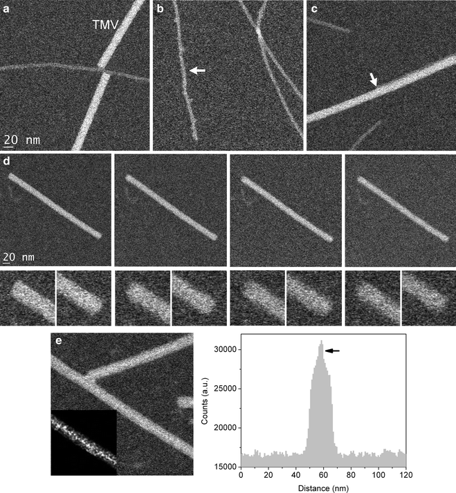
Fig. 2.

Quality assessment of dark-field STEM images. (a) Image with clean fibril, TMV and background regions suitable for STEM mass analysis. (b) Image showing contaminants attached to one of the fibrils (arrow ). (c) Image showing an amyloid fibril attached alongside a TMV virus (see TMV region to the right of the arrow ). The TMV region to the left of the arrow is clean of any attached fibrils. (d) Series of images of TMV at increasing electron dose. Each image was acquired with 3,000 e/nm², so the last (rightmost ) image has an accumulated electron dose four times higher than the first. Bottom panels show zoomed in views of the concave and convex ends of TMV. Images of TMV become less sharp with increasing electron dose. (e) Image illustrating the effect of incomplete washing of specimens. The central cavity of the TMV viruses is filled with buffer salts, which can be seen more clearly in the inset image after smoothing and contrast adjustment (notice the brighter contrast in the center and along the length of the TMV). A line profile across the TMV shows increased intensity near the middle, thus revealing a filled central cavity.

Check the TMV viruses to confirm that the accumulated electron dose is not too high. TMV rods have one end concave and the other convex, but under conditions of high accumulated electron doses these ends lose their sharpness (Fig. 2d).

In addition, check the overall quality of the TMV viruses. First, make sure that the TMV rods appear sharp along their length. TMV with a fuzzy appearance might indicate not only that the electron dose is too high (Fig. 2d), but also that the image is out of focus or that amyloid fibrils are attaching alongside TMV (which we commonly observe in our specimens) (Fig. 2c). Second, check that the central cavity of TMV is not filled with buffer salts or other contaminants, which can be sometimes detected by STEM (Fig. 2e).

Repeat steps 1–5 over different regions of the specimen grid. Samples for STEM mass analysis are not necessarily homogeneous across the entire specimen grid, and as a result some sample regions can be better suited for analysis than others.

3.3 Data Processing and Analysis

HAADF STEM images can be analyzed “automatically” using specialized software to yield the MPL of amyloid fibrils, including PCMass (15) and MASDET (16, 17). Here we present step-by-step instructions for manually carrying out measurements of MPL using standard image processing software (ImageJ). Nonetheless, most of the points addressed below are of general nature and must also be kept in mind when using specialized software.

Select a STEM image containing both sharp and clean TMV and fibrils as explained in Subheading 3.2.3. The image must also be free of contaminants in the background.

Only gold members can continue reading. Log In or Register to continue