Fig. 1.
Schematic of an AFM indentation experiment depicting a probe with a pyramidal tip indenting a cell.
In this chapter, we provide a detailed protocol for measuring the elastic moduli of living cells, which includes calibration of the cantilever spring constant, acquisition of force curves on cells, and data analysis. Throughout the chapter, we include advice and troubleshooting tips based on our own experiences with these measurements. In Chapter 17 of the first edition of Cell Imaging Techniques: Methods and Protocols (27), Costa outlined methods for performing force measurements on cells using the original BioScope™ AFM system from Veeco Instruments (now known as Bruker AXS Inc.). Here, we focus on the more recently developed BioScope™ Catalyst™ AFM system (Bruker AXS Inc.) and provide more specific, step-by-step instructions for acquiring single force curves on cells with the goal of calculating the average elastic modulus of a population of cells. Note that throughout this chapter we have indicated software commands by quotation marks (e.g., “initialize the stage”).
2 Materials
2.1 AFM System
The BioScope™ Catalyst™ AFM system is fully integrated with an inverted optical microscope to enable simultaneous force measurements and optical imaging. The open design of the AFM head permits a direct light path from the condenser to the optical objective for optimal phase contrast and differential interference contrast (DIC) imaging. The open design also facilitates the use of cell culture dishes and easy access to the sample. The following components are supplied with the AFM system:
1.
BioScope™ Catalyst™ head.
2.
Nanoscope V controller.
3.
BioScope™ Catalyst™ Electronics Interface Box (“E-box”).
4.
BioScope™ Catalyst™ baseplate with large NA sample holder plate.
5.
EasyAlign™ for infrared laser alignment.
6.
Joystick for controlling x, y, z motors.
7.
Nanoscope software (version 8.10).
8.
Probe holder for submersion in liquid.
9.
Probe stand for securing probe holder while loading and unloading probes.
10.
Magnetic sample substrate clamps.
2.2 Additional Microscope Components
1.
Nikon Eclipse Ti-E inverted light microscope (Nikon Instruments Inc., Melville, NY) with ×20 or ×40 Ph2 objective for phase imaging (see Note 2).
2.
Controller for microscope shutters (e.g., Lambda 10-3, Sutter Instrument Company, Novato, CA).
3.
Vibration isolation table.
4.
Two computers: one with the Nanoscope software and AFM drivers installed and the other with the optical microscope software and drivers installed.
5.
Digital camera (optional).
6.
Fluorescence lamp (optional).
2.3 Additional Supplies
1.
AFM probes appropriate for contact mode in fluid with spring constants around 0.01–0.2 N/m and a reflective coating on the back side of the cantilever (see Note 3).
2.
Tweezers with non-scratching synthetic tips (e.g., Carbofib tweezers, Aven, Inc., Ann Arbor, MI) to avoid damaging the glass window on the liquid probe holder.
3.
Standard 25 mm × 75 mm microscope slides.
5.
Standard cell culture reagents.
7.
50 mm glass-bottom Petri dishes (WillCo Wells).
8.
Pipette.
9.
Kimwipes® for cleanup.
3 Methods
3.1 Sample Preparation
1.
Seed cells in cell culture dishes or on glass coverslips (see Note 5). We recommend seeding at a cell density that is sub-confluent but greater than 5,000 cells/cm2 to make locating cells easier and to reduce travel time between cells.
2.
Allow cells to adhere and spread (2–24 h) prior to force measurements.
3.2 Cantilever Spring Constant Calibration
The actual spring constant of a cantilever can vary significantly from the nominal spring constant estimated by the manufacturer, and it is important to measure this value before each experiment. Various methods for measuring cantilever spring constants have been reviewed elsewhere (28, 29). We use the Thermal Tune method built into the Nanoscope software, which measures the thermal fluctuations of the cantilever as a function of time, calculates the power spectrum of the fluctuations, fits the chosen peak to a Lorentzian curve, and integrates under the curve to calculate the cantilever spring constant. This measurement should be conducted in air with a clean, dry cantilever, and it first requires measurement of the “deflection sensitivity” (i.e., the conversion factor between cantilever deflection and photodetector voltage) on a material that is very stiff compared to the cantilever, such as glass or tissue culture plastic.
1.
First turn on the computers and then turn on the Nanoscope V controller and the E-box. The optical microscope components should also be turned on.
2.
Open the Nanoscope software, and under experiment type choose “contact mode in fluid.” This will turn the infrared laser on. Do not initialize the stage yet because the laser first needs to be aligned on the AFM probe.
3.
Slide the probe holder for submersion in liquid onto the probe stand. Using tweezers with non-scratching synthetic tips (to protect the glass window on the probe holder), carefully pick up an AFM probe substrate by the sides (see Note 6) and place it on the probe holder with the tip facing up and with the cantilever of interest above the glass window. Push down on the probe stand to raise the spring-loaded clamp and slide the probe under the clamp so that the cantilever is in the center of the glass window. If there are additional cantilevers on the other end of the probe (under the clamp), they will likely be damaged and should not be used.
4.
Stand the AFM head up vertically on the EasyAlign and slide the probe holder onto the z scanner. Lower the AFM head horizontally onto the EasyAlign (without liquid in the dish holder) so that the three legs on the head fit into the three dents in the EasyAlign. Turn the EasyAlign on and adjust the AFM head so that the cantilever is in view, adjusting the focus and brightness knobs as necessary.
5.
Use the beam positioning knobs on the AFM head to move the laser spot onto the end of the cantilever (where the tip is located). Use the horizontal detector positioning knob (−H+) on the AFM head to set the horizontal deflection to 0 and the vertical detector positioning knob (−V+) to set the vertical deflection to a negative number (between −2 and −6 V). The laser sum should be a positive number greater than 2 and should be greatest when the laser is positioned on the cantilever (see Note 7).
6.
With the AFM head still resting on the EasyAlign, follow the prompts in the Nanoscope software to “initialize the stage” and “wake up” the scanners.
7.
Place a clean, dry microscope slide onto the sample holder plate on the microscope stage and secure the slide with the appropriate sample clamp.
8.
Use the Navigation Menu in the Nanoscope software to ensure that the AFM head is near its highest position and then place the head on the stage so that the three legs on the head fit into the three dents on the baseplate.
9.
Use the optical microscope to focus on the top surface of the microscope slide. Using either the joystick or the Navigation Menu in the software, carefully lower the AFM head closer to the glass slide but still far enough away to be out of focus. If the z position of the AFM head is unclear, it is best to stay far away from the glass surface to avoid crashing the probe and z scanner; note that the greater the initial probe-sample separation distance, the more time will be needed to engage.
10.
In the Scan Menu, set the scan size to zero and the deflection setpoint to around 1.5 V. Then in the Engage Menu, use the “slow engage” function to automatically bring the AFM head down to the surface. During this process, the scanner is set to scan mode and the AFM head is lowered to the surface until the vertical cantilever deflection reaches the specified deflection setpoint (see Note 8). Once the deflection setpoint is reached, the tip will start scanning the surface. The default engage settings can be used (“SPM engage step size” = 1 μm, “SPM withdraw step size” = 100 μm), or alternatively, we prefer to use an “SPM engage step size” of 5 μm to speed up the engagement process.
11.
Once the probe is engaged at the surface, switch to the Ramp Menu and raise the AFM head 10 μm by going to “Microscope” in the menu bar and choosing “step motor” or by clicking the “step motor” icon in the RealTime Status Window. Be sure to check the box: “allow stage motion while engaged”.
12.
Look through the optical microscope and check that the cantilever is in view. If necessary, temporarily raise the AFM head another 10–20 μm and adjust the stage using the baseplate positioning knobs (see Note 9).
13.
In the Ramp Menu under the expanded view, choose the following settings: “ramp output” = Z, “ramp size” = 12 μm, “forward and reverse velocities” = 10 μm/s (which corresponds to 0.42 Hz), “number of samples” = 2,048, “Z-closed loop” = ON (see Note 10), “trigger mode” = relative, “data type” = deflection error, “trigger threshold” = 1–2 V (or about 50–100 nm), “start mode” = motor step, and “end mode” = retracted. Adjust the vertical deflection to be around −2 V (see Note 11), and then click the “single ramp” button in the toolbar to acquire a force curve on the glass slide (see Note 12).
14.
In the graph, set channel 1 to “deflection error,” which plots the data as vertical deflection vs. z position. The extension part of the curve should have a flat baseline followed by a sharp, positive slope denoting deflection of the cantilever by the glass surface. The slope of this line gives the “deflection sensitivity” in nm/V, which enables the vertical deflection value to be converted from volts to nanometers. Zoom into the sloped region of the curve by holding “Ctrl” and using the mouse to draw a box around the curve. Then click to the left or right of the graph to drag two red, dashed lines onto the graph and use these lines to mark the boundaries of the sloped region to be fit with a straight line (Fig. 2). Click the “update sensitivity” button in the toolbar to calculate the slope of the line and save this value. Click the magnifying glass button in the bottom left corner of the graph to zoom back out.
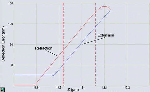
Fig. 2.
Screenshot from the Nanoscope software showing a magnified view of a force curve taken on a glass slide. The extension portion of the curve between the vertical dashed lines is used to calculate the “deflection sensitivity.” For clarity, the extension and retraction curves are labeled, and the font size for the axes has been enlarged.
15.
Bring the AFM head up at least 200 μm by clicking the “withdraw” button several times. Set both the vertical and horizontal deflections to 0 by adjusting the detector positioning knobs on the AFM head and click the “Thermal Tune” button in the toolbar. Do not change the laser beam position (see Note 13).
16.
In the Thermal Tune Menu, check the box for “Lorentzian (Air),” choose the “thermal tune range” of 5–2,000 kHz, enter 1.144 for “deflection sensitivity correction” for v-shaped cantilevers or 1.106 for rectangular cantilevers, and then click the “acquire data” button. Zoom into the largest peak (which should be within the frequency range estimated by the probe manufacturer) and drag red lines onto either side of it to define the boundaries for fitting. Click “fit data” and “calculate spring constant” and then save this value.
3.3 Deflection Sensitivity Calibration in Water
Since the force measurements on cells will be conducted in liquid, the deflection sensitivity must first be recalibrated on a glass slide in water.
1.
Place a 50 mm Petri dish in the dish holder of the EasyAlign and fill it with about 2–3 mL of deionized water.
2.
Stand the AFM head up vertically on the EasyAlign and use a pipette to carefully place one or two drops of deionized water onto the probe. Carefully lay the AFM head down horizontally so that the tip holder is in contact with the water, but only partially submerged. Do not allow liquid to reach the electrical connections between the probe holder and the z scanner.
3.
Turn the EasyAlign on and realign the laser onto the end of the cantilever if necessary. Set the horizontal deflection to 0 and the vertical deflection to around −6 V.
4.
Add a few drops of water to the microscope slide (see Note 4) and place the AFM head onto the stage so that the probe contacts the water and forms a meniscus.
5.
6.
Follow steps 13 and 14 of Subheading 3.2 to update the “deflection sensitivity” in water and save this value.
7.
Withdraw the AFM head at least 300 μm and place it horizontally on the EasyAlign so that the probe is in contact with the water in the dish (see Note 15).
3.4 Force Measurements on Cells
Since physically indenting a cell can stimulate rearrangements of the cytoskeleton and possibly alter cellular mechanical properties (30, 31), we recommend indenting each cell only once and assaying a large number of cells to account for both spatial heterogeneity within a cell as well as cell to cell heterogeneity across the population.
Get Clinical Tree app for offline access
1.
Place the cell culture sample on the microscope stage and secure it with the appropriate magnetic sample clamp. If the sample is on a coverslip, remove the coverslip from the cell culture medium, wick excess medium from the bottom of the coverslip with a Kimwipe®, place it on a microscope slide (preferably hydrophobic), and add a few drops of medium to the top of the coverslip. Do not add too much medium or it will run underneath the coverslip and cause it to float.
2.
Carefully place the AFM head on the microscope stage so that the probe contacts the cell culture medium and forms a meniscus. If the sample is thick, first raise the AFM head further using the joystick or the Navigation Menu to avoid crashing the probe.
3.
Repeat step 5 of Subheading 3.3
 Histochemical Detection of Lipid Droplets in Cultured Cells
Environmental Scanning Electron Microscopy Gold Immunolabeling in Cell Biology
Histochemical Detection of Lipid Droplets in Cultured Cells
Environmental Scanning Electron Microscopy Gold Immunolabeling in Cell Biology
 Colocalization Analysis in Fluorescence Microscopy
 Morphological Analysis of Autophagy
 A Novel Combined Imaging/Morphometrical Method for the Analysis of Human Sural Nerve Biopsies for Clinical Diagnosis
 Environmental Scanning Electron Microscopy in Cell Biology


Related posts:
Histochemical Detection of Lipid Droplets in Cultured Cells
Environmental Scanning Electron Microscopy Gold Immunolabeling in Cell Biology
Colocalization Analysis in Fluorescence Microscopy
Morphological Analysis of Autophagy
Environmental Scanning Electron Microscopy in Cell Biology
Stay updated, free articles. Join our Telegram channel
Full access? Get Clinical Tree
