Modeling of the Spine

consists of vertices $\{{\mathbf {v}}_{j}^{i}|j=1,\ldots ,V_i\}$ and triangles.

Further prior knowledge can be encoded into the surface meshes by labelling the individual triangles. An example is given in Fig. 1a. This labelling allows to easily derive certain vertebra characteristics directly from the mesh, e.g., distance between vertebral body surfaces. Finally, important anatomical landmarks can be annotated in the mesh as shown in Fig. 1b. As both surface labelling and landmark setting only need to be done once during model generation, manual annotation is typically done.

Fig. 1

Illustration of additional prior knowledge encoded into the shape models, a Labelling of anatomical regions. b Annotated anatomical landmarks

The surface descriptions can be embedded into a multi-resolution representation with different levels of complexity. In [20], three levels of polygonal mesh catalogues were created to speed up processing and allow for optimal convergence using a coarse-to-fine strategy during registration.

2.2 Statistical Shape Modelling

From the initial vertebra surface representations, we can build statistical vertebra shape models by adapting the surfaces to a set of images. During patient individualization, we carefully preserve the established vertex distribution of the generated vertebra surface representation. By using the adaptation algorithm from Chapter 5, the topology remains unchanged and the vertex distribution is constrained to be similar to the respective reference mesh, so that the

th landmark of the

th mesh lies at approximately the same anatomical position for all cases. After segmentation of all vertebrae in a set of training images, a Procrustes co-registration is performed and finally a point distribution model can be obtained. In the following, we keep however only the mean surface models ${\mathbf {s}}_i$ for each vertebra. Thus, the overall geometrical spine model can be expressed as $\mathbf S = \{{\mathbf {s}}_{1},\ldots ,{\mathbf {s}}_{L}\}$ with

if all vertebrae are considered.

2.3 Vertebra Coordinate System

In addition to the surface representation, each vertebra model carries its own local vertebra coordinate system (VCS). This allows to express relative location and orientation of the individual vertebrae. In order to have similar definition of the VCS for the individual vertebrae along the spine, a VCS is typically defined by invariant object characteristics and different definitions have been proposed. In [23], we derived the VCS of all vertebra from the surface mesh representation including the labelling of anatomical regions (see Fig. 1a). For the vertebrae C3 to L5, the VCS was defined in the same way since these vertebrae show similar shape characteristics. The definition of the VCS was based on three object-related simplified representations: a cylinder fit to the vertebral foramen, the middle plane of the upper and lower vertebral body surfaces, and the sagittal symmetry plane of the vertebra (see Fig. 2). The definition of the VCS was as follows: The origin of the VCS was located in the mid-vertebral plane at the centre of the vertebral foramen. The normal vector of the middle plane defined the ${\mathbf {z}}_{\mathrm {VCS}}$ -axis, the ${\mathbf {x}}_{\mathrm {VCS}}$ -axis was defined by the orthogonal component of the normal vector of the symmetry plane and the ${\mathbf {z}}_{\mathrm {VCS}}$ -axis. The cross product of ${\mathbf {z}}_{\mathrm {VCS}}$ -axis and ${\mathbf {x}}_{\mathrm {VCS}}$ -axis resulted in the ${\mathbf {y}}_{\mathrm {VCS}}$ -axis [23]. For the unique definition of the VCS for C1 and C2, other characteristics were chosen. A vertex subset was chosen containing the vertices belonging to the inferior articular faces and the anterior tubercle. The axes of the specific VCSs are given by the covariance analysis of the subset. The eigenvector corresponding to the largest eigenvalue of the covariance matrix points to the lateral direction defining the ${\mathbf {x}}_{\mathrm {VCS}}$ -axis, the second eigenvector pointing towards the anterior tubercle gives the ${\mathbf {y}}_{\mathrm {VCS}}$ -axis, and finally, the third eigenvector points towards the direction of the spinal canal denoting the ${\mathbf {z}}_{\mathrm {VCS}}$ -axis. The barycentre of the subset defines the origin of the VCS.

Fig. 2

Invariant features of vertebrae used to define a VCS: Cylinder fit to vertebral foramen (a), middle plane of upper and lower vertebral body surface (b) as well as sagittal symmetry plane (c)

Alternatively, the VCS for the thoracic and lumbar vertebrae was derived in [21] from six anatomical landmarks defined in the mesh (4 pedicle tips and 2 on the vertebral body, as depicted in Fig. 1b).

2.4 Gradient Model

For vertebra detection, we further created generalised Hough transform models of each vertebra. The generalised Hough transform (GHT) [6] is a robust and powerful method to detect arbitrary shapes in an image undergoing geometric transformations. During GHT learning, description of the shape is encoded into a reference table also called R-table. Its entries are vectors pointing from the shape boundary to a reference point being commonly the gravity centre of the shape. During detection, the gradient orientation is measured at each edge voxel of the new image yielding an index for an entry of the R-table. Then, the positions pointed by all vectors under this entry are incremented in an accumulator array. Finally, the shape is given by the highest peak in the accumulator array. Usually, the GHT is trained for one single reference shape of an object class. In addition to specific GHT models for C1 to L5 we build general cervical, thoracic and lumbar GHT models. The general models can be applied if the field of view of the available image is unknown while the more specific models can be used if some indication for a certain area of the spine is given.

Fig. 3

Gradient model representation of sixth thoracic vertebra in axial and sagittal view showing the model points. The model has been created from ten samples

For model generation, shape models adapted to a set of training images are superimposed based on the VCSs and the obtained aligned shapes are used to build up the R-table. Note that the orientation is not considered during GHT learning since all shapes were aligned via the respective VCS. In contrast to the above mentioned shape models, the GHT models do not only contain shape information but also gradient information. A gradient model for the sixth thoracic vertebra can be seen in Fig. 3. For more details about the gradient models, we refer to [24].

2.5 Appearance Model

Vertebra appearance models in this case are represented as average intensity volumes inside a bounding box around each vertebra without explicitly modeling the vertebra’s shape. The information covered in the model about expected appearance in the direct neighbourhood of each vertebra can be used to identify vertebrae in an image by comparing the similarity between model and image content. For model generation, shape models need to be adapted to a set of training images. Mean intensity volumes are then generated by aligning volumes around corresponding vertebrae and averaging the intensity values. Alignment is performed by registration of the vertebra shape models to their respective model space. The obtained transformations can then be applied on the respective voxel positions. Location and pose of the object in the volumes are expressed by the VCSs of the mean vertebra models that were used for alignment. Exemplarily, the appearance model of the sixth thoracic vertebra is shown in Fig. 4. Inter-patient variability becomes obvious by blurry object boundaries whereas the particular objects are still clearly delimited. More details can be found in [24].

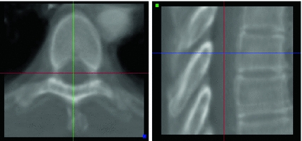
Fig. 4

Appearance model of sixth thoracic vertebra in axial and sagittal view generated from ten training images. The volume has a sample distance of 0.5 mm in each direction. The cross gives the origin of the VCS

3 Articulated Models

In the previous section, each vertebra has been represented seperately by a set of detailed models. However, in order to model the overall constellation of the spine, the articulation between the individual vertebrae has to be considered. In this section, we first introduce a general representation of the articulated spine model in Sect. 3.1. Based on this representation, statistical modeling of the spine can be done and two different methods are proposed in Sects. 3.2 and 3.3. In each case, it is furthermore shown how the articulated model can be individualized to a new patient.

3.1 Model Definition

As defined in Sect. 2, the geometric model of the spine is defined as ${\mathbf {S}} = \{{\mathbf {s}}_1, \ldots , {\mathbf {s}}_L\}$ consisting of an interconnection of $$L$$

objects. Each local shape ${\mathbf {s}}_i$ is represented as a triangulated mesh including a VCS to rigidly register each object to its upper neighbor.

The resulting rigid transforms are stored for each inter-object link. Hence, an articulated deformable model (ADM) is represented by a series of local inter-object rigid transformations $$T_i$$

(translation and rotation) between neighbouring vertebrae resulting in

$\begin{aligned} {\mathbf {A}}=[T_1, T_2, \ldots , T_{L-1}]\,. \end{aligned}$

(1)

While ${\mathbf {A}}$ covers the individual inter-object transformations, the global shape of the spine shape can be expressed by converting ${\mathbf {A}}$ into an absolute representation

$\begin{aligned} {\mathbf {A}}_{\mathrm {abs}}=[T_1, T_1 \circ T_2, \ldots , T_1 \circ T_2 \circ \ldots \circ T_{L-1}] \end{aligned}$

(2)

using recursive compositions. The respective transformations are expressed in the VCS of the lower object.

The relationship between the shape model ${\mathbf {S}}$ and the ADM is that the articulation vector ${\mathbf {A}}$ controls the position and orientation of the object constellation ${\mathbf {S}}$ . The ADM can achieve deformation by modifying the vector of rigid transformations, which taken in its entirety, performs a global deformation of the spine [22].

The rigid transformations are the combination of a rotation matrix ${\mathbf {R}}$ and a translation vector ${\mathbf {t}}$ , while scaling is not considered. We formulate the rigid transformation $T = \{{\mathbf {R}}, {\mathbf {t}}\}$ of a triangular mesh model as ${\mathbf {y}} = {\mathbf {R}}{\mathbf {x}} + {\mathbf {t}}$ where ${\mathbf {x}}, {\mathbf {y}}, {\mathbf {t}} \in \mathfrak {R}^3$ . Composition is given by $T_1 \circ T_2 = \{{\mathbf {R}}_1{\mathbf {R}}_2,{\mathbf {R}}_1{\mathbf {t}}_2 + {\mathbf {t}}_1\}$ .

Alternatively, a rigid transformation can be fully described by an axis of rotation supported by a unit vector ${\mathbf {u}}$ and an angle of rotation $\theta$ . The rotation vector ${\mathbf {r}}$ is defined as the product of ${\mathbf {u}}$ and $\theta$ . Thus, a rigid transformation can be expressed as $T = \{\theta {\mathbf {n}}, {\mathbf {t}}\} = \{{\mathbf {r}}, {\mathbf {t}}\}$ . The conversion between the two representations is simple, since the rotation vector can be converted into a rotation matrix using Rodrigues’ formula (see Appendix for more details).

3.2 Linear Model

3.2.1 Model Generation

In order to capture variations of the spine curve, statistics need to be applied on the articulated model. As defined in the previous section, the spine is expressed as a vector of rigid transformation and there is no addition or scalar multiplication defined between them. Thus, as the representation no longer belongs to a vector space, conventional statistics can not be applied. However, rigid transformations belong to a Riemannian manifold and Riemannian geometry concepts can be efficiently applied to generalize statistical notions to articulated shape models of the spine. The mathematical framework described in the following has been introduced by Boisvert et al. and explained, e.g., in [8–10].

Following the statistics for Riemannian manifolds, the generalization of the usual mean called the Fr ${\acute{\mathrm {e}}}$ chet mean can be defined for a given distance measure as the element $\mu$ that minimizes the sum of the distances with a set of elements $x_{0},\ldots ,x_{N}$ of the same manifold ${\mathcal {M}}$ :

$\begin{aligned} \mu = \mathrm{arg\,min }_{x\in {\mathcal {M}}} \sum _{i=0}^N d(x, x_i)^2{\,\text {.}} \end{aligned}$

(3)

Since the mean is given as a minimization, the gradient descent method can be performed on the summation obtaining

$\begin{aligned} \mu _{n+1} = \mathrm{Exp }_{\mu _n}\Biggl ( \frac{1}{N}\sum _{i=0}^N \mathrm{Log }_{\mu _n}(x_i)\Biggr ){\,\text {.}} \end{aligned}$

(4)

The functions Exp and Log are respectively the exponential map and the log map associated with the distance $$d(x, y)$$

. The exponential map projects an element of the tangent plane on the manifold ${\mathcal {M}}$ and the log map is the inverse function.

The intuitive generalization of the variance is the expectation of the squared distance between the elements $$x_i$$

$\begin{aligned} \sigma ^2 = E[d(\mu , x)^2] = \frac{1}{N}\sum _{i=0}^{N}{d(\mu , x_i)^2}. \end{aligned}$

(5)

The covariance is usually defined as the expectation of the matricial product of the vectors from the mean to the elements on which the covariance is computed. The expression for Riemannian manifolds can thus be given by using again the Log map [8]:

$\begin{aligned} \varSigma _{xx} = E[{\mathrm {Log}}(\mu ^{-1}x)^T{\mathrm {Log}}(\mu ^{-1}x)] = \frac{1}{N}\sum _{i=0}^{N}{\mathrm {Log}}_\mu (x){\mathrm {Log}}_\mu (x)^T. \end{aligned}$

(6)

To use the Riemannian framework defined by Eqs. 3–6, a suitable distance needs to be defined first to find the structure of the geodesics on the manifold. For this purpose, we rely on the representation of transformation as a rotation vector as defined in Sect. 3.1. With this representation, the left-invariant distance definition between two rigid transformations can be defined [9]:

$\begin{aligned} d(T_1, T_2) = N_\omega (T_2^{-1} \circ T_1) \quad \mathrm{with }\quad N_\omega (T)^2 = N_\omega (\{{\mathbf {r}}, {\mathbf {t}}\})^2 = ||{\mathbf {r}}||^2 + ||\omega {\mathbf {t}}||^2 \end{aligned}$

(7)

where $\omega$ is used to weight the relative effect of rotation and translation, ${\mathbf {r}}$ is the rotation vector, and ${\mathbf {t}}$ the translation vector. An appropriate value for the weight factor $\omega$ in the case of the spine is found to be 0.05 [8].

Fig. 5

First, second and third eigenmode of the statistical model on transformation between the local coordinate systems defined on the 12 thoracic vertebrae. Each row shows the mean transformation model $\mu$ and the mean plus a particular eigenmode weighted by $\pm 3\sqrt{\lambda _i}$ with $$i=1,...,3$$

. The resulting transformations are applied to mean shape models based on 18 patient data sets, a $\mu -3\sqrt{\lambda _1}\phi _1$ , b Mean $\mu$ , c $\mu +3\sqrt{\lambda _1}\phi _1$ , d $\mu -3\sqrt{\lambda _2}\phi _2$ , e Mean $\mu$ , f $\mu +3\sqrt{\lambda _2}\phi _2$ , g $\mu -3\sqrt{\lambda _3}\phi _3$ , h Mean $\mu$ , i $\mu +3\sqrt{\lambda _3}\phi _3$

Finally, exponential and logarithmic map associated with the defined distance are the conversions between the rotation vector and the rotation matrix combined with a scaled version of the translation vector [8]

$\begin{aligned} {\mathrm {Exp}}_{Id}(T) = \left| \begin{array}{c} {\mathbf {R}}(r) \\ \omega ^{-1} {\mathbf {t}} \end{array} \right. \ \ \mathrm{and }\ \ \ {\mathrm {Log}}_{Id}(T) = \left| \begin{array}{c} r({\mathbf {R}}) \\ \omega {\mathbf {t}} \end{array} \right. \,. \end{aligned}$

(8)

Given the articulated model of the spine is expressed as the multivariate vector ${\mathbf {A}}^T=[T_1, T_2, \ldots , T_L]^T$ from Eq. 1 of $$L$$

rigid transformations, we obtain for the mean and the covariance

$\begin{aligned} \mu = \begin{pmatrix} \mu _1\\ \mu _2\\ \vdots \\ \mu _L\\ \end{pmatrix} \quad \mathrm{and } \quad \varSigma = \begin{pmatrix} \varSigma _{T_1 T_1}&{} \varSigma _{T_1 T_2}&{} \ldots &{} \varSigma _{T_1 T_{L}}\\ \varSigma _{T_2 T_1}&{} \varSigma _{T_2 T_2}&{} \ldots &{} \varSigma _{T_2 T_{L}}\\ \vdots &{} \vdots &{} &{} \vdots \\ \varSigma _{T_{L} T_1} &{} \varSigma _{T_{L} T_2} &{} \ldots &{} \varSigma _{T_{L} T_{L}} \end{pmatrix}{\,\text {.}} \end{aligned}$

(9)

With Eq. 9, the formulation for the linear statistical spine model is given. In order to reduce the dimensionality of the model, principal component analysis (PCA) can be performed on the covariance matrix. As an example, Fig. 5 shows the first three eigenmodes after applying PCA to the statistics of transformations between the 12 thoracic vertebrae obtained from 18 patients.

3.2.2 Model Adaption

The statistical spine model can be used to support image segmentation. It allows to consider the object constellation during segmentation instead of separate segmentation of the individual vertebrae, thus going from single object to multi-object segmentation. Such a framework has been presented in [25] for the segmentation of the spine in CT. Its general idea is to follow a two-scale adaptation approach. During a global adaptation step, the individual vertebrae are at first roughly positioned in the image. Afterwards, exact segmentation of the vertebrae is achieved by adaptation of the respective vertebra shape models. In this section, we focus on the adaptation of the global model, while details for deformable surface mesh adaptation are basically explained earlier in Chap. 5.

The idea of global adaptation is to determine the inter-object transformations $$T_k$$

by minimizing an energy term $$E(T_k)$$

where an external energy $E_{\mathrm {ext}}(T_k)$ drives the vertebrae towards image features, while an internal energy $E_{\mathrm {int}}(T_k)$ restricts attraction to a former learned constellation model

$\begin{aligned} E(T_k) = E_{\mathrm {ext}}(T_k)+\alpha E_{\mathrm {int}}(T_k) {\,\text {.}} \end{aligned}$

(10)

The parameter $\alpha$ controls the trade-off between both energy terms which are explained in the following.

The external energy attracts each vertebra towards its corresponding image structures. Thus, we first need to define a feature function such as

$\begin{aligned} F_{i}({{\mathbf {x}}_{i}})=-{{\mathbf {n}}_{i}}^T \nabla I({\mathbf x}_{i}) \frac{g_{\mathrm {max}}( g_{\mathrm {max}}+\left\| \nabla I({{\mathbf {x}}_{i}})\right\| )}{g^2_{\mathrm {max}}+\left\| \nabla I({{\mathbf {x}}_{i}})\right\| ^2} \end{aligned}$

(11)

that evaluates for each vertebra independently the match between the vertebra surface mesh and the underlying image structure. The feature function is evaluated for each triangle of the surface mesh at the position of the triangle barycentre ${\mathbf {x}}_{i}$ . The image gradient $\nabla I({\mathbf {x}}_i)$ is projected onto the face normal ${\mathbf {n}}_{i}$ of each triangle and damped by $g_\mathrm {max}$ . The feature values of all triangles are summed up providing one value per vertebra for the current position.

The search for a new vertebra position is performed by testing various discrete locations inside a local neighborhood around a given position. For that purpose, a cartesian grid inside a bounding box around the current estimated vertebra location is defined. In order to not only cope with translations but also rotations, the original object is rotated in discrete steps around all axes obtaining $$M$$

rotation matrices ${\mathbf {R}}_m$ . At each of the $$N$$

grid positions, the feature function from Eq. 11 is evaluated for the corresponding surface mesh translated by ${\mathbf {t}}_n$ as well as its $$M$$

rotated versions. Due to the frequent presence of local minima, the exhaustive search of transformation parameters is preferred to other optimization strategies. It has to be noted again that this search aims at finding a new vertebra position while the original surface model is not deformed yet.

The transformation resulting in the highest feature strength determines the new position of the object:

$\begin{aligned} {\mathrm {arg\,\,max}}_{{\mathbf {R}}_m, {\mathbf {t}}_n}\sum _{i \in T}F_{i}({\mathbf {R}}_m{\mathbf {x}}_{i}+{\mathbf {t}}_n){\,\text {,}} \end{aligned}$

(12)

where

is the number of triangles per mesh.

After finding the most promising positions for a pair of neighboring objects $$m$$

and

, we can define the global external energy for the corresponding $$k$$

th transformation using the distance measure between transformations as introduced in Eq. 7:

$\begin{aligned} E_{\mathrm {ext}_k} = d(\tilde{T}^{-1}_{\mathrm {VCS}_m}\cdot \tilde{T}_{\mathrm {VCS}_n},T_k)^2 \end{aligned}$

(13)

where ${\tilde{T}}_{\mathrm {VCS}_m}$ and ${\tilde{T}}_{\mathrm {VCS}_n}$ are the transformations of the corresponding VCSs at the new positions to the world coordinate system. Thus, $\tilde{T}^{-1}_{\mathrm {VCS}_m}\!\cdot \, \tilde{T}_{\mathrm {VCS}_n}$ gives the transformation between the corresponding VCSs.

Driving the model towards high image features as performed by the external energy is restricted by the internal energy to prevent false attraction. The internal energy preserves similarity of the ensemble towards an earlier learned constellation model. This is expressed by defining for each transformation $$T_k$$

$\begin{aligned} E_{\mathrm{int }_k} = d\Bigl (\mathrm{Exp }_{\mu _k}\Biggl (\sum _{i=1}^t b_i {\mathbf {c}}_{i,k}\Biggr ), T_k\Bigr )^2 \quad \mathrm{with } \quad {\mathbf {b}} = {\mathbf {C}}^T({\mathrm {Log}}_{\mu }{\mathbf {A}}^T)\ \end{aligned}$

(14)

where the matrix of the individual eigenvectors $\mathbf {c}_i$ is denoted as ${\mathbf {C}}$ and $$b_i$$

is the coordinate of the weight vector ${\mathbf {b}}$ associated with the $$i$$

th principal component. The internal energy penalizes differences between the model and the current constellation. The closest constellation to the model is determined by projecting the given constellation ${\mathbf {A}}^T$ in the sub-space defined by the principal components.

After calculating the respective energy terms, the final transformations $$T_k$$

between the individual objects are determined by minimizing

$\begin{aligned} E(T_k) = d(T_{\mathrm {ext}_k},T_k)^2+\alpha \cdot d(T_{{\mathrm {int}}_k},T_k)^2 \end{aligned}$

(15)

for each object separately. The transformations $T_{{\mathrm {ext}}_k}$ and $T_{{\mathrm {int}}_k}$ are obtained from the external and internal energy, respectively. The final transformation $T_{k_\mathrm {opt}}$ is found using a Downhill-Simplex optimizer. As the representation of the ensemble as a consecution of rigid transformations requires a reference VCS, the vertebra with the highest feature strength is taken as the reference in each iteration.

After positioning the vertebra models using the global model adaptation, a local non-rigid free-form deformation similar to Chap. 5 of the individual surface meshes can be carried out. In order to improve segmentation, all vertebrae are adapted simultaneously with the individual shapes interacting on each other to prevent misadaptations. This has been realized in [25] by introducing a collision detection into feature search and decreasing the feature strength the deeper a target point lies inside another mesh.

3.3 Manifold Embedding

3.3.1 Model Generation

As an alternative to the linear statistical model proposed in the previous section, low-dimensional manifold embedding of the articulated model has been proposed in [20, 21].

For non-linear embedding, we rely on the absolute vector representation ${\mathbf {A}}_{\mathrm {abs}}=[T_1, T_1 \circ T_2, \ldots , T_1 \circ T_2 \circ \ldots \circ T_{L-1}]$ as given in Eq. 2. Let us now consider $$N$$

articulated shape models expressed by the feature vectors $\mathbf{A }_\mathrm{abs }^{i}$ , of dimensionality $$D$$

. The aim is to create a low-dimensional manifold consisting of $$N$$

points ${\mathbf {Y}}_{i}, {\mathbf {Y}}_{i}\in \mathfrak {R}^{d}, i\in [1,N]$ where $d\ll D$ based on [35]. In such a framework, if an adequate number of data points is available, then the underlying manifold ${\mathcal {M}}$ is considered to be “well-sampled”. Therefore, it can represent the underlying population structure. In the sub-cluster corresponding to a pathological population, each point of the training set and its neighbours would lie within a locally linear patch as illustrated in Fig. 6.

Fig. 6

Representation of inter-vertebral transformations in manifold space

The main limitation of embedding algorithms is the assumption of Euclidean metrics in the ambient space to evaluate similarity between sample points. Thus, similar to Sect. 3.2, a metric in the space of articulated structures is defined that accommodates for anatomical spine variability and adopts the intrinsic nature of the Riemannian manifold geometry allowing us to discern between articulated shape deformations in a topological invariant framework. For each point, the $$K$$

closest neighbours are selected using a distortion metric which is particularly suited for geodesics. The metric $d_{\mathrm {M}}(\mathbf{A }_\mathrm{abs }^{i},\mathbf{A }_\mathrm{abs }^{j})$ estimates the distance of articulated models $$i,j$$

. The distance measure for absolute representations can therefore be expressed as a sum of articulation deviations

$\begin{aligned} d_M(\mathbf{A }_\mathrm{abs }^{i},\mathbf{A }_\mathrm{abs }^{j}) = \sum _{k=1}^{L} d_M(T_{k}^{i},T_{k}^{j}) =\sum _{k=1}^{L}\Vert \mathbf{t }_{k}^{i}-\mathbf{t }_{k}^{j}\Vert +\sum _{k=1}^{L}d_{G}(\mathbf{R }_{k}^{i},\mathbf{R }_{k}^{j}). \end{aligned}$