Monitoring of Syndesmophyte Growth in Ankylosing Spondylitis Using Computed Tomography

Fig. 1

Example of syndesmophyte growth from baseline (BL) to year 1 (Y1) visible on CT reformations but not on radiographs

To overcome the limitations of radiographic methods, we designed a computer algorithm that quantitatively measures syndesmophyte volumes in the 3D space of CT scans [7, 8].

2 The Algorithm

The complete algorithm, summarized in Fig. 2, has of three main parts. First, vertebral bodies are segmented using a 3D multi-stage level set method. Triangular meshes representing the surfaces of the segmentations are made. The 3D surfaces shown in Fig. 2 are triangular meshes obtained from our segmentation results. The vertebral surfaces of corresponding vertebrae are then registered. The purpose of the registration is to extract the syndesmophytes of both vertebrae using the same reference level. Syndesmophytes are cut from the vertebral body using the end plate’s ridgeline as the reference level.

Fig. 2

Overview of the complete algorithm

2.1 Segmentation of the Vertebral Bodies

Many image processing segmentation techniques have previously been applied to the extraction of vertebral bodies in CT [9–11]. For our algorithm, we chose to use level sets for their flexibility [12]. Flexibility is essential in our application as syndesmophytes can deform the normal vertebral structure in unexpected ways. Level sets are evolving contours encoded as the zero level set of a distance function $\psi \left( {\vec {x},t} \right)$ . Points that verify $\psi \left( {\vec {x},t} \right) =0$ form the contour. The contour is made to evolve using equations such as [13]:

$\begin{aligned} \frac{d\psi }{dt}=\alpha g\left( {\vec {x}} \right) c\left| {\nabla \psi } \right| +\beta g\left( {\vec {x}} \right) \kappa \left| {\nabla \psi } \right| +\gamma \nabla g\left( {\vec {x}} \right) \nabla \psi . \end{aligned}$

(1)

The three terms on the right-hand side of the equation respectively control the expansion or contraction of the contour (velocity $$c$$

), the smoothness of the contour using the mean curvature $\kappa$ and the adherence of the contour to the boundary of the object to be segmented. The parameters $\alpha , \beta$ and $\gamma$ allow the user to weight the importance of each term. The spatial function $g\left( {\vec {x}} \right)$ , often called speed function, is derived from the images to be segmented and contains information about the objects’ boundaries. The design of the speed function is crucial for the success of the segmentation. Depending on the specific needs of the application, information on the object’s boundary can be based on image gradient, Laplacian or any other relevant feature. Details about our level set implementation have been fully described [7].

2.2 Segmentation of the Vertebral Body Ridgelines

The segmentation of vertebral body ridgelines is a preliminary step to both the registration stage (Sect. 2.3) and the syndesmophyte extraction stage (Sect. 2.4). The vertebral body ridgelines provide the landmarks that aid the registration process and the reference level from which syndesmophytes are cut. We extract the ridgelines from the triangular meshes representing the surfaces of the vertebrae using the same level set as Eq. 1, but transposed from the Cartesian domain of rectangular grids to the domain of a surface mesh.The most important adjustment is to design a suitable speed function. While in the usual image grids of CT scans the relevant features are grey level gradients, on a surface mesh, the useful features are curvature measures (the vertebral body surface is more curved at the ridgelines than on the end plates). The curvature measure we used is curvedness ( $$C$$

) [14]:

$\begin{aligned} C=\sqrt{\frac{\kappa _1^2 +\kappa _2^2 }{2}} \end{aligned}$

(2)

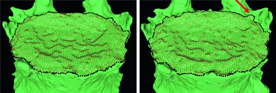
where $\kappa _1$ and $\kappa _2$ are the principal curvatures.The speed function ensures that the level set contour expands in the center of the end plates and stops at the ridgelines. The most complete description of the mesh level set can be found in [7].

Fig. 3

End plate (red) and ridgeline (black) segmentation at baseline (left) and year 1 (right)

Figure 3 shows an example of ridgeline segmentation at baseline and year 1. Bone above the ridgeline will be labeled as syndesmophyte. Some small differences between the 2 ridgelines are visible (arrow). Although the difference can seem minor, it can lead to differences in syndesmophyte volume measurements. Such differences would not be due to real syndesmophyte growth. Because real growth may be small, it is important to reduce the error coming from ridgeline discrepancies. That is the motivation behind the next step, registration, which aligns the 2 vertebral surfaces so that only one of the ridgelines needs to be used as the reference level from which to cut syndesmophytes.

Only gold members can continue reading. Log In or Register to continue