Fig. 1.
Two shape complexes composed by a pseudo cortex, divided into a black and green area, and a red pseudo fiber bundle. A single diffeomorphism could not capture the differences in structural connectivity and put in correspondence both structures. A double diffeomorphism would first move the fiber bundle from the left to the right gyrus and then it would change the shape of the gyri, producing an accurate matching (Color figure online).
In order to deal with the considerable amount of fibers resulting from tractography algorithms, we rely on the approximation scheme introduced in [4]. Fiber bundles are approximated with weighted prototypes represented as “tubes”. They are chosen among the fibers and their radius is related to the number of fibers approximated. This new representation is based on the metric of weighted currents [4], an extension of the framework of currents. As usual currents, it does not require point-correspondence between fibers or fiber-correspondence between bundles. Two fibers modelled as weighted currents are considered similar if their pathways are alike and their endpoints are close to each other. This metric makes therefore possible to match correctly also the extremities of two fiber bundles and not only their central part as in usual currents. This is fundamental in order to retrieve the connectivity changes at the end of the first diffeomorphism.
The atlas is estimated using a generative statistical model similar to the one in [2] adapted to double diffeomorphisms. The proposed Bayesian model uses similar priors as in [1] which enables to automatically estimate the noise variance of each structure and the covariance matrix of the deformation parameters for both diffeomorphisms. The set of noise variances represent a trade-off between each data-term and the two deformation regularity terms.
In Sect. 2, we first introduce how we model the brain structures summarizing the framework of weighted currents and weighted prototypes. We then present the proposed framework of double diffeomorphism and include it into a Bayesian atlas construction method. In Sect. 3, we first apply our new scheme to a toy matching example comparing its performance with the one of a single diffeomorphism. Then, we build an atlas with the proposed technique using real data.
2 Bayesian Double Diffeomorphic Atlas Construction
2.1 Object Representation
Gray Matter. Gray matter objects are modelled as 3D surfaces, where we assume vertex correspondence across subjects. The norm of the difference between two meshes is defined as the sum of squared differences between pair of vertices.
White Matter. Fiber bundles are modelled as weighted currents [4]. Let X and Y be two fibers which can be modelled as polygonal lines of Q and Z segments respectively. We define  for X and
  for Y as the vectors containing the coordinates of their extremities. The inner product between these two tracts in the framework of weighted currents is given by:

 where
where  and
and  are the centres and tangent vectors of the segments of X and Y respectively and
  ,
,  and
and  are Gaussian kernels whose bandwidth is fixed by the user. The last one defines the range of interaction between the points of X and Y, as in usual currents, while
  and
and  set the distances at which extremities of the fibers are considered close. Two fibers are similar if their pathways are alike and if their extremities are close to each other. The space of weighted currents is a vector space, which implies that a fiber bundle B is seen as the sum of its fibers
  :
:  . This makes possible to easily compare two fiber bundles, which do not need to have the same number of fibers, by expanding the inner product
  chosen among the fibers [4]. The prototype
  is modelled as a weighted current and its weight
  is linked to the number of fibers approximated. This approximation scheme is controlled by the residual error:
  in the space of weighted currents. It permits to reduce the number of fibers to analyse while preserving connectivity (location of the fiber endpoints on the gray matter) and geometry (pathway of the fibers).
for X and for Y as the vectors containing the coordinates of their extremities. The inner product between these two tracts in the framework of weighted currents is given by: where and are the centres and tangent vectors of the segments of X and Y respectively and , and are Gaussian kernels whose bandwidth is fixed by the user. The last one defines the range of interaction between the points of X and Y, as in usual currents, while and set the distances at which extremities of the fibers are considered close. Two fibers are similar if their pathways are alike and if their extremities are close to each other. The space of weighted currents is a vector space, which implies that a fiber bundle B is seen as the sum of its fibers : . This makes possible to easily compare two fiber bundles, which do not need to have the same number of fibers, by expanding the inner product chosen among the fibers [4]. The prototype is modelled as a weighted current and its weight is linked to the number of fibers approximated. This approximation scheme is controlled by the residual error: in the space of weighted currents. It permits to reduce the number of fibers to analyse while preserving connectivity (location of the fiber endpoints on the gray matter) and geometry (pathway of the fibers).2.2 Double Diffeomorphic Deformation
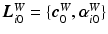
Let N be the number of subjects and M the number of objects. All structures of subject i can be seen as a shape complex  which is modelled as a double deformation of a common template complex
  plus a residual noise
  where
where  ,
,  and the upper indices W and G refer to the White and Gray matter respectively:
The first deformation  deforms the white matter keeping fixed the gray, thus modeling the changes in the relative position between white and gray matter objects. The second deformation
  matches both gray and white matter (the latter already deformed by
  ). Both deformations depend on subject i and they are the last deformation of a flow of diffeomorphisms built by integrating a time-varying vector field
  (t
(t  [0, 1], x
 ) (see [5] for details). The two vector fields
  and
and  are defined by two different sets of control points
  and
and  shared among the whole population, and by two sets of 3D vectors, called momenta,
  and
and  linked to the control points and specific to each subject i:
  and
and 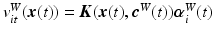 , where
  represents a block matrix of Gaussian kernels with equal fixed width for both deformations. Control points and momenta evolve in time according to the differential equations:
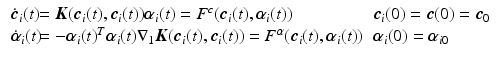
This system of ODEs is valid for both diffeomorphisms:  =
= ,
,  and it can be summarized as
  . The last diffeomorphisms
  and
and  are completely parametrized by the initial conditions of the systems:
 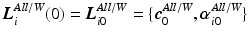 . Thus, in order to deform the template complex
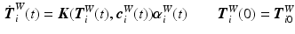
  , we first integrate forward in time
  starting from
  and we use these values to deform only the white objects of the template complex (
 ) integrating forward in time:
The deformed white matter template, together with the un-deformed gray matter template ( ), are then used as starting point for the second deformation All:
  .
.  is integrated forward in time starting from
  and the global template
  is deformed using a similar equation as Eq. 3. Omitting the index i for clarity purpose, the composition is computed as:
which is modelled as a double deformation of a common template complex plus a residual noise where , and the upper indices W and G refer to the White and Gray matter respectively:(1)
deforms the white matter keeping fixed the gray, thus modeling the changes in the relative position between white and gray matter objects. The second deformation matches both gray and white matter (the latter already deformed by ). Both deformations depend on subject i and they are the last deformation of a flow of diffeomorphisms built by integrating a time-varying vector field (t [0, 1], x ) (see [5] for details). The two vector fields and are defined by two different sets of control points and shared among the whole population, and by two sets of 3D vectors, called momenta, and linked to the control points and specific to each subject i: and , where represents a block matrix of Gaussian kernels with equal fixed width for both deformations. Control points and momenta evolve in time according to the differential equations:(2)
=, and it can be summarized as . The last diffeomorphisms and are completely parametrized by the initial conditions of the systems: . Thus, in order to deform the template complex , we first integrate forward in time starting from and we use these values to deform only the white objects of the template complex () integrating forward in time:(3)
), are then used as starting point for the second deformation All: . is integrated forward in time starting from and the global template is deformed using a similar equation as Eq. 3. Omitting the index i for clarity purpose, the composition is computed as:2.3 Optimization Procedure
We show here how to estimate the template complex  and the deformation parameters
 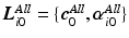 ,
,  which characterize respectively the invariants and the variability of the set of anatomical configurations. This is performed using a Bayesian framework like in [1, 2, 17]. Assuming independence between the variables, we model
  and
and  as multivariate Gaussian variables:

 ,
, 

 as well as the residual noise
  :
: 

 and
and 

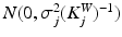


![$$\exp \left[ -\frac{1}{2\sigma _{j}^2}||\varPi (S_{ij}^W - \phi _i^{All}(\phi _i^W(T_j^W))) ||^2_{W_{\Lambda j}^*}\right] $$](/wp-content/uploads/2016/09/A339424_1_En_21_Chapter_IEq77.gif) where
where  refers to the size of the j-th grid on which both the shapes and the template of the j-th white matter structure are projected in order to define probability density functions (space of weighted currents is infinite). Moreover we add priors on
  ,
,  and
and  using Inverse Wishart distributions:
 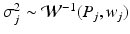 ,
, 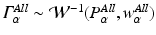 ,
, 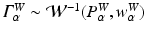 where the matrices
  ,
,  and the scalars
  ,
, ,
,  ,
,  are hyper-parameters. Both the template complex
  and the control points
  and
and  have a uniform prior distribution. The parameters
 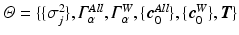 should be estimated considering
  and
and  as latent variables and
  as observations using, for instance, Monte Carlo sampling procedures (as in [17]). This process would be very time-consuming and we have thus opted for a faster MAP estimation, where
  and
and  are considered as parameters
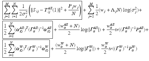
  . The (minus) log posterior distribution of
  given the observations
  is equal to:
 Stable Overlapping Replicator Dynamics for Multimodal Brain Subnetwork Identification
 PET Reconstruction with Sparse Image Representation and Anatomical Priors
 Gaussian Process-Based Modelling and Prediction of Image Time Series
 Multimodal Joint Generative Model of Brain Data
 Trajectory and Progression Score Estimation from Voxelwise Longitudinal Imaging Measures: Application to Amyloid Imaging
 Frames for Heart Fiber Reconstruction


and the deformation parameters , which characterize respectively the invariants and the variability of the set of anatomical configurations. This is performed using a Bayesian framework like in [1, 2, 17]. Assuming independence between the variables, we model and as multivariate Gaussian variables: , as well as the residual noise : and where refers to the size of the j-th grid on which both the shapes and the template of the j-th white matter structure are projected in order to define probability density functions (space of weighted currents is infinite). Moreover we add priors on , and using Inverse Wishart distributions: , , where the matrices , and the scalars ,, , are hyper-parameters. Both the template complex and the control points and have a uniform prior distribution. The parameters should be estimated considering and as latent variables and as observations using, for instance, Monte Carlo sampling procedures (as in [17]). This process would be very time-consuming and we have thus opted for a faster MAP estimation, where and are considered as parameters . The (minus) log posterior distribution of given the observations is equal to:Related posts:
Stable Overlapping Replicator Dynamics for Multimodal Brain Subnetwork Identification
PET Reconstruction with Sparse Image Representation and Anatomical Priors
Stay updated, free articles. Join our Telegram channel
Full access? Get Clinical Tree
