Understanding normal anatomy of the hip is important for diagnosing its pathology. MR arthrography is more sensitive for the detection of intra-articular pathology than noncontrast MR imaging. Important elements of the osseous structures on MR imaging include the alignment and the marrow. Acetabular ossicles may be present. Normal variations involving the cartilage include the supra-acetabular fossa and the stellate lesion. Important muscles of the hip are the sartorius, rectus femoris, iliopsoas, gluteus minimus and medius, adductors, and hamstrings. The iliofemoral, ischiofemoral, and pubofemoral ligaments represent thickenings of the joint capsule that reinforce and stabilize the hip joint. Normal variations in the labrum include labral sulcus and absent labrum. The largest nerves in the hip and thigh are the sciatic nerve, the femoral nerve, and the obturator nerve.
Key Points
- •
Understanding normal anatomy is important for diagnosing pathology of the hip.
- •
MR arthrography is more sensitive for the detection of intra-articular pathology than noncontrast MR imaging.
- •
Important components of hip anatomy include the osseous structures, cartilage, muscles and tendons, capsular ligaments, labrum, nerves, and vessels.
Imaging the hip
Hip pain is a common complaint, especially in athletes, and it has a broad differential diagnosis. MR imaging has improved the radiologist’s ability to diagnose causes of hip pain, especially soft tissue pathology.
The hip joint is difficult to image because it is not oriented in the standard axial, coronal, and sagittal planes of the body, and there is significant variation in hip joint orientation from person to person. Acetabular version, for example, can range from −10.8 to +22.1 degrees.
At the authors’ institution, MR imaging is performed on 1.5- and 3-T scanners using a phased-array surface coil. One fluid-sensitive sequence is obtained with a large field of view that includes the proximal femurs, the pelvis, and the sacrum. The remaining sequences use a small field of view focused on the symptomatic hip and are acquired in the standard axial, coronal, and sagittal imaging planes. They also use an oblique axial imaging plane (also known as the “sagittal oblique” imaging plane by some authors ), oriented parallel to the long axis of the femoral neck, to evaluate for labral tears and femoroacetabular impingement. These images are prescribed using a coronal localizer image that includes the superior labrum and the transverse acetabular ligament; the oblique axial images are then acquired perpendicular to the line that connects these two structures ( Fig. 1 ). The imaging parameters used at the authors’ institution on the 1.5- and 3-T MR imaging scanners are detailed in Tables 1 and 2 .
| Sequence | TR | TE | TI | NEX | Matrix | ST × Sk | FOV | Flip Angle |
|---|---|---|---|---|---|---|---|---|
| Coronal FMPIR | 3800 | 45 | 150 | 1 | 320 × 192 | 5 × 6 | 360 | 90 |
| Axial PD | 1933 | 27 | 2 | 320 × 256 | 4 × 5 | 180 | 90 | |
| Coronal T1 | 483 | 10 | 1 | 384 × 224 | 4 × 5 | 200 | 90 | |
| Coronal T2 FS | 4150 | 76 | 1.5 | 320 × 224 | 4 × 5 | 200 | 90 | |
| Sagittal PD | 2267 | 44 | 1 | 320 × 224 | 4 × 5 | 200 | 90 | |
| Oblique axial PD FS | 2583 | 35 | 1 | 512 × 256 | 4 × 5 | 180 | 90 |
| Sequence | TR | TE | TI | NEX | Matrix | ST × Sk | FOV | Flip Angle |
|---|---|---|---|---|---|---|---|---|
| Coronal FMPIR | 4250 | 48 | 200 | 1 | 320 × 192 | 4 × 4.4 | 360 | 120 |
| Axial PD | 2730 | 9 | 1 | 256 × 256 | 4 × 4.4 | 200 | 140 | |
| Coronal T1 | 931 | 15 | 2 | 384 × 307 | 4 × 4.6 | 199 | 140 | |
| Coronal T2 FS | 3070 | 60 | 1 | 256 × 256 | 4 × 5 | 200 | 150 | |
| Sagittal PD | 3500 | 43 | 2 | 384 × 307 | 4 × 4.4 | 199 | 170 | |
| Oblique axial PD FS | 4000 | 69 | 2 | 256 × 154 | 3 × 3 | 200 | 150 |
The authors also inject intra-articular contrast to perform MR arthrography. The intra-articular contrast distends the joint, separates the soft tissue structures, and increases the contrast resolution, all of which help to increase the conspicuity of intra-articular pathology, such as labral tears, osteocartilaginous bodies, and osteochondral and cartilage defects.
Using fluoroscopic guidance, a 22-gauge needle, and an anterior or anterolateral approach, the authors position the needle within the joint and inject 10 to 12 mL of a 1:250 mixture of dilute gadolinium (10 mL of a mixture consisting of 0.4 mL of gadopentetate dimeglumine [Magnevist; Bayer Healthcare Pharmaceuticals, Wayne, NJ] diluted in 50 mL of normal saline, 5 mL of iopamidol 41% [Isovue-M-200; Bracco Diagnostics, Princeton, NJ], and 5 mL of preservative-free lidocaine 1%). They target the superolateral aspect of the femoral head/neck junction to minimize the possibility of injecting into the femoral vessels or the iliopsoas tendon sheath. The imaging digital detector may be angled laterally by approximately 15 degrees to further avoid puncturing these structures and also to create a trajectory approximately perpendicular to the target injection location. Alternatively, if the digital detector cannot rotate, the toes can be taped inward, which places the hip at approximately 15 degrees of internal rotation. Care is taken to remove all bubbles from the syringe, tubing, and needle, because air bubbles create MR imaging blooming artifact, which may mimic intra-articular osteocartilaginous bodies or otherwise obscure pathology. The capacity of the hip joint varies from 8 to 20 mL. During the injection, they use fluoroscopy to look for a “rings of Saturn” pattern of contrast around the femoral neck to confirm that the injection is intra-articular ( Fig. 2 ). When the injection is complete, the patient is brought directly to the MR imaging scanner; imaging should commence within 30 minutes of contrast injection to maximize joint distention and to minimize contrast resorption. All MR arthrography sequences use a small field of view focused on the injected hip. The imaging parameters used at the authors’ institution for MR arthrography on the 1.5- and 3-T MR imaging scanners are detailed in Tables 3 and 4 .
| Sequence | TR | TE | NEX | Matrix | ST × Sk | FOV | Flip Angle |
|---|---|---|---|---|---|---|---|
| Axial T2 FS | 2250 | 53 | 3 | 320 × 192 | 4 × 4 | 160 | 180 |
| Coronal T1 | 660 | 14 | 2 | 320 × 192 | 4 × 4 | 160 | 180 |
| Coronal T1 FS | 563 | 12 | 2 | 320 × 224 | 4 × 4 | 160 | 180 |
| Coronal T2 FS | 2250 | 53 | 3 | 320 × 192 | 4 × 4 | 160 | 180 |
| Sagittal T1 FS | 550 | 11 | 2 | 320 × 192 | 3.5 × 3.5 | 160 | 180 |
| Oblique axial T1 FS | 600 | 15 | 2 | 320 × 192 | 3.5 × 3.5 | 160 | 180 |
| Sequence | TR | TE | NEX | Matrix | ST × Sk | FOV | Flip Angle |
|---|---|---|---|---|---|---|---|
| Axial T2 FS | 3500 | 82 | 2 | 384 × 307 | 4 × 4 | 159 | 150 |
| Coronal T1 | 663 | 15 | 1 | 448 × 336 | 4 × 4 | 160 | 140 |
| Coronal T1 FS | 570 | 15 | 1 | 448 × 318 | 4 × 4 | 160 | 140 |
| Coronal T2 FS | 4320 | 82 | 3 | 384 × 311 | 4 × 4 | 159 | 150 |
| Sagittal T1 FS | 640 | 13 | 2 | 448 × 318 | 3.5 × 3.5 | 160 | 170 |
| Oblique axial T1 FS | 550 | 14 | 1 | 448 × 318 | 3.5 × 3.5 | 160 | 140 |
Imaging the hip
Hip pain is a common complaint, especially in athletes, and it has a broad differential diagnosis. MR imaging has improved the radiologist’s ability to diagnose causes of hip pain, especially soft tissue pathology.
The hip joint is difficult to image because it is not oriented in the standard axial, coronal, and sagittal planes of the body, and there is significant variation in hip joint orientation from person to person. Acetabular version, for example, can range from −10.8 to +22.1 degrees.
At the authors’ institution, MR imaging is performed on 1.5- and 3-T scanners using a phased-array surface coil. One fluid-sensitive sequence is obtained with a large field of view that includes the proximal femurs, the pelvis, and the sacrum. The remaining sequences use a small field of view focused on the symptomatic hip and are acquired in the standard axial, coronal, and sagittal imaging planes. They also use an oblique axial imaging plane (also known as the “sagittal oblique” imaging plane by some authors ), oriented parallel to the long axis of the femoral neck, to evaluate for labral tears and femoroacetabular impingement. These images are prescribed using a coronal localizer image that includes the superior labrum and the transverse acetabular ligament; the oblique axial images are then acquired perpendicular to the line that connects these two structures ( Fig. 1 ). The imaging parameters used at the authors’ institution on the 1.5- and 3-T MR imaging scanners are detailed in Tables 1 and 2 .
| Sequence | TR | TE | TI | NEX | Matrix | ST × Sk | FOV | Flip Angle |
|---|---|---|---|---|---|---|---|---|
| Coronal FMPIR | 3800 | 45 | 150 | 1 | 320 × 192 | 5 × 6 | 360 | 90 |
| Axial PD | 1933 | 27 | 2 | 320 × 256 | 4 × 5 | 180 | 90 | |
| Coronal T1 | 483 | 10 | 1 | 384 × 224 | 4 × 5 | 200 | 90 | |
| Coronal T2 FS | 4150 | 76 | 1.5 | 320 × 224 | 4 × 5 | 200 | 90 | |
| Sagittal PD | 2267 | 44 | 1 | 320 × 224 | 4 × 5 | 200 | 90 | |
| Oblique axial PD FS | 2583 | 35 | 1 | 512 × 256 | 4 × 5 | 180 | 90 |
| Sequence | TR | TE | TI | NEX | Matrix | ST × Sk | FOV | Flip Angle |
|---|---|---|---|---|---|---|---|---|
| Coronal FMPIR | 4250 | 48 | 200 | 1 | 320 × 192 | 4 × 4.4 | 360 | 120 |
| Axial PD | 2730 | 9 | 1 | 256 × 256 | 4 × 4.4 | 200 | 140 | |
| Coronal T1 | 931 | 15 | 2 | 384 × 307 | 4 × 4.6 | 199 | 140 | |
| Coronal T2 FS | 3070 | 60 | 1 | 256 × 256 | 4 × 5 | 200 | 150 | |
| Sagittal PD | 3500 | 43 | 2 | 384 × 307 | 4 × 4.4 | 199 | 170 | |
| Oblique axial PD FS | 4000 | 69 | 2 | 256 × 154 | 3 × 3 | 200 | 150 |
The authors also inject intra-articular contrast to perform MR arthrography. The intra-articular contrast distends the joint, separates the soft tissue structures, and increases the contrast resolution, all of which help to increase the conspicuity of intra-articular pathology, such as labral tears, osteocartilaginous bodies, and osteochondral and cartilage defects.
Using fluoroscopic guidance, a 22-gauge needle, and an anterior or anterolateral approach, the authors position the needle within the joint and inject 10 to 12 mL of a 1:250 mixture of dilute gadolinium (10 mL of a mixture consisting of 0.4 mL of gadopentetate dimeglumine [Magnevist; Bayer Healthcare Pharmaceuticals, Wayne, NJ] diluted in 50 mL of normal saline, 5 mL of iopamidol 41% [Isovue-M-200; Bracco Diagnostics, Princeton, NJ], and 5 mL of preservative-free lidocaine 1%). They target the superolateral aspect of the femoral head/neck junction to minimize the possibility of injecting into the femoral vessels or the iliopsoas tendon sheath. The imaging digital detector may be angled laterally by approximately 15 degrees to further avoid puncturing these structures and also to create a trajectory approximately perpendicular to the target injection location. Alternatively, if the digital detector cannot rotate, the toes can be taped inward, which places the hip at approximately 15 degrees of internal rotation. Care is taken to remove all bubbles from the syringe, tubing, and needle, because air bubbles create MR imaging blooming artifact, which may mimic intra-articular osteocartilaginous bodies or otherwise obscure pathology. The capacity of the hip joint varies from 8 to 20 mL. During the injection, they use fluoroscopy to look for a “rings of Saturn” pattern of contrast around the femoral neck to confirm that the injection is intra-articular ( Fig. 2 ). When the injection is complete, the patient is brought directly to the MR imaging scanner; imaging should commence within 30 minutes of contrast injection to maximize joint distention and to minimize contrast resorption. All MR arthrography sequences use a small field of view focused on the injected hip. The imaging parameters used at the authors’ institution for MR arthrography on the 1.5- and 3-T MR imaging scanners are detailed in Tables 3 and 4 .