MR Imaging of the Skeletal Musculature: From Static Measures to a Dynamic Assessment of the Muscular (Loco-) Motion

where L is the length in the ‘deformed’ state. Strain is dimensionless and represents the fractional or percentage change in dimension.

It is also possible to define the instantaneous strain defined by:

${\upvarepsilon}_{1{\text D}} \left( {\text{t}} \right) = {\text{L}}\left( {\text{t}} \right)-{\text{L}}_{0} \left( {\text{t}} \right)/{\text{L}}_{0} \left( {\text{t}} \right)$

It should be noted that there are two types of strain defined based on the reference length. If the reference length is the initial length, the strain is called Lagrangian strain. On the other hand, if the reference length (e.g., in the instantaneous strain) is a previous time point (rather than a static reference at the initial time point), it is then termed as the natural or engineering strain.

1D strain rate, ε_SR, is defined as:

${{\upvarepsilon}}_{\text{SR}} = \frac{\Updelta \varepsilon }{\Updelta t} = \frac{{\left( {{\raise0.7ex\hbox{${\Updelta L}$} \!\mathord{\left/ {\vphantom {{\Updelta L} {L_{0} }}}\right.\kern-0pt} \!\lower0.7ex\hbox{${L_{0} }$}}} \right)}}{\Updelta t} = \frac{{\left( {{\raise0.7ex\hbox{${\Updelta L}$} \!\mathord{\left/ {\vphantom {{\Updelta L} {\Updelta t}}}\right.\kern-0pt} \!\lower0.7ex\hbox{${\Updelta t}$}}} \right)}}{{L_{0} }} = \frac{{\Updelta {\text{v}}}}{{L_{0} }}$

where ∆v is the velocity gradient and ε_SR has the units of sec⁻¹. Strain rate has the same direction as the strain (negative strain during shortening and positive strain during elongation). Velocity encoded-phase contrast MRI provides a direct measure of velocity and this strain rates can be directly measured from them.

4.1 Two-Dimensional Strain Rate Mapping

The 2D spatial gradient of the velocity vector, L is first calculated as:

$L = \left[ {\frac{{\partial {\text{u}}}}{{\partial {\text{x}}}}\frac{{\partial {\text{u}}}}{{\partial {\text{y}}}};\;\frac{{\partial {\text{v}}}}{{\partial {\text{x}}}}\frac{{\partial {\text{v}}}}{{\partial {\text{y}}}}} \right]$

where u and v are the x and y components of the velocity vector. Next, the symmetric part of the strain rate tensor is calculated from: ${{\upvarepsilon}}_{{ 2 {\text{D}}}} = 0.5\left( {L + L^{T} } \right)$ . The 2×2 strain rate tensor, ε_2D, is then diagonalized to obtain the eigenvalues and eigenvectors. The positive and negative values at each voxel representing the local expansion and contraction, respectively, are usually stored as separate images.

The same procedure is applied to map 2D strains except that the 2D velocity vector (u, v) in the above equation will be replaced with the 2D deformation vector (where the deformation vector is estimated for a given voxel with respect to a reference position). The extension to 3D will involve the velocity vector and deformation vector in 3D and the spatial derivatives will have t estimated in all three (x, y, and z) directions.

5 MR Compatible Device for MR Measurements

Dynamic MRI studies of the musculoskeletal (MSK) system require MR compatible devices to enable the acquisition of displacement/velocity sensitive images under different contraction conditions. Sinha et al. report the design and development of an MR-compatible, computer-controlled, foot-pedal device capable of operating inside the bore of an MR scanner at both 1.5 and 3 Tesla (Sinha et al. 2012). This device enabled dynamic acquisitions to map the changes in strain and shape during passive and neutral conditions and at different activation levels, load, and ankle joint angle under dynamic conditions of plantarflexion or dorsiflexion use. Figure 1 shows the schematic of the setup including the positioning of the foot pedal and subject in the scanner. The foot was secured with a Velcro strap and subjects could exert force against the foot-pedal plate during plantarflexion (concentric contraction) or dorsiflexion (eccentric contraction), or exert no force at all for passive movement. Provision for isometric contraction was also made with the foot pedal anchored at a neutral 90^°. A Fabry–Perot optical strain gauge bonded to the foot pedal and the force proportional output voltage was projected in real-time to provide feedback and modulate the contraction from the subject. The output is also used to generate a trigger pulse for gating the acquisition during isometric contractions.

Fig. 1

a Schematic diagram of the experimental setup. The experimental components are interconnected via coaxial cables. Work output of the motor was transmitted to the foot pedal via hydraulic fluid (water) in high-pressure tubing. The tube passed from the console room to the MRI scanning room through a waveguide in the wall. Force data from the foot pedal was projected onto the white front surface of the magnet through a projector for realtime feedback to the subject. An electronic trigger signal was transmitted directly from the motor to the ECG port of the scanner at a preselected point of each contraction cycle for gated image acquisition. b Schematic of the foot pedal apparatus: assembly of all CAD parts. Different components are annotated. c Photo of the actual foot-pedal device. The motor is shown in the lower left connected to the stainless steel piston-cylinder, hydraulic tubing coiled on the right, connected to the white, nonmetallic piston-cylinder which goes inside the magnet bore. The piston can be seen connected to the foot pedal in the upper middle part of the picture. (Reprinted with permission from Sinha et al. 2012 )

A modification of this device for dynamic images of the thigh has also been reported (Sinha et al. 2013). Zhong et al. have reported an MR compatible device to perform a full range of elbow flexion–extension in order to map displacements and strains in the biceps brachii muscle (Zhong et al. 2008). Image acquisition was gated to the onset of elbow flexion using a photodiode circuit.

6 Velocity Encoded-Phase Contrast (VE-PC) MR Musculoskeletal Imaging

The first study of musculoskeletal imaging using velocity encoded-phase contrast imaging was reported by Drace and Pelc (Drace and Pelc 1994a, b, c, d). In the latter study, they successfully tracked the in vivo motion of the human forearm muscles during finger extension and flexion, and the muscles of the anterior and posterior compartment of the lower extremity with varying levels of resistance for ankle dorsi- and plantarflexion. They also measured the strain of the myotendinous junction and tendon using an in situ model and motion phantom apparatus. The motion phantom apparatus consisted of a pair of rotating disks in the axial plane, and on one disk the belly of a gastrocnemius muscle was sutured and on the other disk, the distal end of the tendon of the gastrocnemius muscle was sutured. A grid was inked onto the tendon, muscle, and muscle–tendon junction and motion was videotaped with specific grid points on the tendon, muscle, and muscle–tendon junction being digitized. The changes in position of these grid points allowed calculation of strain. These strain values from video images were compared to those derived from the velocity-encoded cine phase MRI technique. The MRI technique involved measuring the velocities of the same ROI’s and then performing successive iterations of movement of the ROI (by multiplying the velocity over the time delay of the phase to get the next position of the same region of interest). The tendon and myotendionous junction strain as determined from the MR imaging experiments was plotted as a function of the strain determined from the video with a correlation coefficient being 0.992 for the myotendinous junction and 0.987 for the tendon (Drace and Pelc 1994b).

Lingamneni et al. measured the motion of a rotating phantom and averaged the trajectories using the MRI-measured velocity data both forward and backward in time from the starting point (Lingamneni et al. 1995). The motion of the phantom was tracked using custom-built algorithms through a complete rotation to an accuracy of two pixels. They also explored the forward and backward integration techniques to measure true trajectories of another rotating phantom. By using the MRI-measured velocity data of points on the phantom, they found that the measured (integrated) and true trajectories agreed to within 3.3 %. The velocity encoded-phase contrast MRI technique has also been used to study the motion of skeletal structures such as the patella (Sheehan et al. 1999; Shellock et al. 1999).

Based on cine phase contrast imaging studies, Pappas et al. reported nonuniform shortening along some muscle fascicles during low load elbow flexion (Pappas et al. 2002). In this study, they calculated displacements of square ROIs from the velocity measurements and 1D strain was determined by calculating the length change between the ROIs placed along the muscle fascicles. These results were later confirmed by finite element model predictions that nonuniform strains can arise from complex features of muscle architecture (Blemker et al. 2005).

A number of studies based on MRI for either velocity or displacement mapping of the lower extremity muscle have been reported. These studies show that the MRI is a promising tool for exploring the architectural features as well as muscle function under different types of muscle activation. Many subtle aspects of the velocity and strain distribution in different muscles can be determined which in turn, allows a deeper understanding of muscle physiology and the potential modifications to these patterns under altered conditions or disease states.

6.1 Soleus

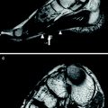
Finni et al. reported the first comprehensive study of the distribution of strain along the soleus aponeurosis tendon during isometric contractions at 20 and 40 % MVC (Finni et al. 2003a). Displacement and strain in the apparent Achilles tendon and in the aponeurosis were calculated from cine phase-contrast MRI; the apparent Achilles tendon lengthened 2.8 and 4.7 % in 20 and 40 % maximal voluntary contraction, respectively. Nonuniformity in aponeurosis strain was reported with the midregion of the aponeurosis, below the gastrocnemius insertion, lengthening by 1.2 and 2.2 %, while the distal aponeurosis shortened by 2.1 and 2.5 %, respectively. Finni et al. postulated that the nonuniformity in aponeurosis strain within an individual was due to the presence of active and passive motor units along the length of the muscle, causing variable force along the measurement site. Force transmission along intrasoleus connective tissue was also considered as a significant source of nonuniform strain in the aponeurosis. A closely related paper by the same group confirmed the strong relationship between the complex 3D structure of the muscle–tendon system of the human soleus and the intramuscular distribution of tissue velocities during in vivo isometric contractions (Finni et al. 2003b). The proximal region of the muscle is unipennate, whereas the midregion has a radially bipennate hemicylindrical structure, and the distal region is quadripennate. Tissue velocity mapping showed that the highest velocity regions overlay the aponeuroses connected to the Achilles tendon (Fig. 2). These are located on the anterior and posterior surfaces of the muscle. The lowest velocities overlay the aponeuroses connected to the origin of the muscle and are generally located intramuscularly. The heterogeneity in the dynamics is attributed by the authors to a combination of an uneven spatial distribution of the motor units that are recruited and the physical structures within the muscle. The heterogeneity parallels the 3D of the muscle–tendon unit, suggesting that further detailed studies of muscle structure are essential for a better understanding of muscle function.

Fig. 2

Cine phase-contrast MR images provide both anatomy (a) and velocity (b) image sequences. These sagittal images (and data in c–e) were taken from the beginning of the contraction during early force rise. In b, the dark and light gray shades represent high velocities in the proximal and distal direction, respectively. Contour velocity maps of the soleus during 20 (c) and 40 % (d) MVC further illustrate the velocity distributions and their dependence on load. The negative velocities represent movement proximally. Positive velocities are not shown in these plots for clarity. e velocity distribution across the soleus muscle taken from midmuscle at the level of the diamond arrows shown in b–d. The midmuscle moves distally, whereas the anterior and posterior edges of the muscle move proximally. f a simple model of part of the soleus muscle in relaxed and contracted conditions illustrating the relative movement of the aponeuroses (thick arrows) and consequent rotation of the muscle fibers. Rotation of the fibers while the interaponeuroses distance is kept constant results in a smaller change in fiber length (ΔL _f) than in tendon length (ΔL _t). Force vectors placed on the anterior soleus (relaxed scheme) illustrate the idea that longitudinally (F _f) and laterally (F _la) transmitted forces relative to the fiber orientation produce a net force (F _net) in the proximal direction to produce proximal tissue movements that supplement fiber length changes in shortening contractions. Force vectors placed on the posterior soleus show that the intramuscular pressure (F _imp) counteracts the fiber force component (F _fx) that would move the aponeuroses closer together. (Reprinted with permission from Finni et al. 2003b)

In order to further understand the correlation of structure to function, the same group explored the structure/function of the soleus muscle in another study. Hodgson et al. provide a detailed comprehensive analysis of the soleus muscle structure and the correlation to function (Hodgson et al. 2006). High resolution images of the soleus muscle from the Visible Human Dataset (available from the National Library of Medicine), magnetic resonance images (MRI), and cadaver studies revealed a complex 3D connective tissue structure populated with pennate muscle fibers. Tracking of these structures through multiple images revealed a regular organization that paralleled the expected orientation of muscle fibers. Figure 3 shows the images reconstructed from the Visible Human dataset and the directions of the muscle fibers inferred from the direction of the intramuscular connective tissue.

Fig. 3

Axial and computer reconstructed sagittal and coronal images from the Visible Human Dataset. The levels of the three axial images on the left (Axial a, c, e ) are shown in the sagittal image using color-coded lines. The orientation of the sagittal image is shown by vertical lines in the axial images. Similarly, the orientations of the coronal and axial images on the right (Axial b, d ) are color coded. The green lines outline the soleus muscle and the dashed light blue lines identify the major intramuscular connective tissue structures. In the proximal leg, the dashed light blue lines distinguish the anterior compartment of the soleus muscle (Axial a, b). The arrows show the orientation of the bands of white tissue that probably correspond to fascicle orientation. The arrowheads indicate the more proximal end of the fascicles. Note that the fascicles may not be oriented along the plane of the coronal or sagittal sections. The dark bands across the sagittal and coronal images indicate missing data. (Reprinted with permission from Hodgson et al. 2006)

An important contribution of the paper by Hodgson et al. is the attempt to link the inhomogeneity of the velocity distribution patterns in the soleus to the muscle structure including to the connective tissue components. One striking feature was the high velocities observed near the posterior aponeurosis and median septum and the low, or even reverse, velocities near the anterior aponeurosis (Fig. 4). The maximum velocities were observed in regions overlying the aponeuroses connected to the Achilles tendon. This was the case for both the posterior soleus aponeurosis and the median septum, which was also connected to the Achilles tendon. Thus, the pattern of intramuscular movement during a muscle contraction corresponded to muscle fibers shortening and rotating as the interdigitating aponeuroses of origin and insertion slid longitudinally relative to each other. Hodgson et al. also inferred that the distribution of the connective tissue (more concentration of noncontractile material in the central regions of the muscle) should result in the appropriate curvature of muscle fibers (Hodgson et al. 2006).

Fig. 4

Axial images to show the relationship between the leg structures and the velocities recorded during isometric contractions. Each row illustrates data from different levels of the calf musculature. a Velocities in the superior–inferior direction during early force development. Speckled areas in the cortical bone and tendon are noise due to low signal levels from these tissues. b Cortical bone and connective tissue are shown in black and superimposed on the velocity images. Note the correspondence between the distribution of velocities and connective tissues within several muscles. c The morphological images used to identify bone and connective tissue. d The morphological images with the soleus muscle and its major connective tissue components identified. Note that the regions near the soleus aponeurosis of insertion (posterior aponeurosis and median septum) had faster velocities than regions close to the aponeurosis of origin (anterior aponeurosis). Note also that this subject activated the deep plantarflexors (DPF) and peroneus muscle (Per), shown by the higher velocities in the area to the left of the fibula. (Reprinted with permission from Hodgson et al. 2006)

6.2 Medial Gastrocs

Kinugasa et al. also reported an anomalous behavior of the MG (medial gastrocnemius) superficial and deep aponeurosis during isometric plantarflexion at 20 and 40 % of MVC. Positive strain (lengthening) occurred in both ends of the deep aponeurosis and in the proximal region of the superficial aponeurosis (Kinugasa et al. 2008). In contrast, negative strain (shortening) was observed in the middle region of the deep aponeurosis and in the distal region of the superficial aponeurosis. Consistent with this shortening of the deep aponeurosis length along the proximal–distal axis was expansion of the aponeuroses in the medial–lateral and anterior–posterior directions in the cross-sectional plane. It is concluded that at low to moderate force levels of isometric contraction, regional differences in strain occur along the proximal–distal axis of both aponeuroses, and some regions of both aponeuroses shorten (Fig. 5). This paper also evaluated the spin tag and phase contrast imaging methods and confirmed that the two methods provide comparable accuracy of displacement measures (Fig. 6).

Fig. 5

(Left column) Strain distribution along the superficial and deep aponeuroses. a average strain distribution along the superficial and deep aponeuroses during 20 (top) and 40 % (bottom) MVC from eight subjects. Positive and negative strain indicate lengthening and shortening, respectively. Values are means. ∗P < 0.05 versus ROI 1; ≠P < 0.05 versus ROI 2; †P < 0.05 versus ROI 3; _P < 0.05 versus ROI 11; aP < 0.05 versus from ROI 3 to ROIs 8, 10, and 11; bP < 0.05 versus ROIs 2, 4, and 10; cP < 0.05 versus ROIs 2–9; ¶P < 0.05, 20 versus 40 % MVC. b model of strain distribution along the proximal–distal axis of both aponeuroses. This model resulted from the strain during 40 % MVC. Dashed lines indicate location of aponeurosis lengthening, and thick solid lines indicate location of aponeurosis shortening. Thin solid lines are the original length of the aponeurosis, i.e., where strain is undetectable. (Reprinted with permission from Kinugasa et al. 2008)

Fig. 6

(Right column) Validation of displacement as determined from PC MRI by comparison with spin-tag experiment. a representative oblique–sagittal spin tagging and PC images during phase 6, which correspond to the peak torque. ROIs are prescribed graphically along both the superficial and deep aponeuroses. b displacement at three different points along the superficial and deep aponeuroses during the first 10 phases is compared between the PC and spin-tagged data. The single-pixel resolution of the spin-tag data results in steps in the displacement curves, whereas the subpixel resolution of the PC imaging provides smoother curves. The displacement measurements show good correlation (r = 0.89 for superficial aponeurosis and r = 0.89 for deep aponeurosis). (Reprinted with permission from Kinugasa et al. 2008)

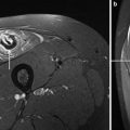
In a continuing series of experiments, Kinugasa et al. further explored the symmetry of muscle fiber deformation (Kinugasa et al. 2012). Constant volume considerations of the deforming muscle predicts that if the fibers lengthen, then the cross-sectional area should decrease. In-plane area measurements along segments of the MG and determination of fiber length changes from phase contrast MRI data allowed deduction of the through-plane deformation. Kinugasa et al. established the asymmetry in fascicle cross-section deformation for both passive and active muscle fibers with a ~22 % in-plane and ~6 % through-plane fascicle thickness change. They postulate that the fiber deformations have functional relevance, not only because they affect the force production of the muscle itself, but also because they affect the characteristics of adjacent muscles by deflecting their line of pull.

Shin et al. showed that PC-MRI allows extraction of parameters beyond velocity, displacement, and strain; these additional parameters enable further characterization of muscle performance and highlight muscle heterogeneity (Shin et al. 2009). The latter paper reports on the intramuscular fascicle-aponeuroses dynamics of the human medial gastrocnemius during plantarflexion and dorsiflexion of the foot. They determined intrafascicular strain defined as the ratio of strain in the fascicle segment at the insertion to strain at its origin. This ratio was nonuniform along the proximo-distal axis of the muscle, increasing from the proximal to distal direction (Fig. 7).

Fig. 7

Left Intrafascicular end-to-end strain ratio for all subjects showing significant regional differences but no difference between the passive and eccentric mode. Values are mean ± SD; n = 12 (distal), 30 (mid), and 12 (proximal). (Reprinted with permission from Shin et al. 2009)

Only gold members can continue reading. Log In or Register to continue