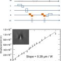
Hervé SAINT-JALMES1, Hélène RATINEY2 and Olivier BEUF2 1 LTSI, Inserm, Université de Rennes, France 2 CREATIS, CNRS, Inserm, INSA Lyon, Université Claude Bernard Lyon 1, France The demonstration of the nuclear magnetic resonance (NMR) phenomenon in condensed matter in 1946 (Bloch 1946; Purcell et al. 1946) certainly stems from significant progress accrued during the previous decade and in particular during the war with the development of radars and radiofrequency technology. Today, a similar consideration can be made for magnetic resonance imaging (MRI), where technological progress contributes significantly to the improvement of measurement instrumentation and therefore to the quality of signal and images produced by these devices. Such progress paves the way for imaging techniques that are not exclusively qualitative but also quantitative. This introductory chapter concisely describes MRI principles and the main components of an MRI scanner, in particular those responsible for the generation of magnetic fields and signal acquisition. Schematically, several steps are required to obtain a localized spectrum or an image (see Figure 1.1): In the following, we will focus on recalling the physical principles of MRI along with the associated technological solutions and their implementation (Saint-Jalmes 2022) up to a general overview of quantitative MRI approaches that are amply presented in this book. Figure 1.1. Sequence of four key steps of an MRI scan of an organ, with a fifth step of image/spectrum reconstruction and extraction of quantified parameters In NMR and MRI, the denomination of magnetic field B is commonly used. From a physical point of view, B is a fundamental quantity, similar to the electric field E in electrostatics (Gié et al. 1976). In the past, the mathematical analogy between vectors E and H led to H being called the magnetic field, with B being then referred to as magnetic induction. The latter term will not be used in this work, although it is still widely used. NMR makes use of the magnetic properties of nuclei having a non-zero spin hI. Among nuclei with such a feature, the most commonly studied are the hydrogen nucleus (1H or proton), phosphorus-31 (31P), sodium-23 (23Na), fluorine-19 (19F) and carbon-13 (13C) (see Chapter 9). In a nucleus with a spin number I (integer or half-integer), the magnetic nuclear moment μ is aligned with the spin moment, such that μ = γħI, where γ, called the gyromagnetic ratio, is a characteristic constant of the nucleus of interest and ħ is the reduced Planck’s constant h/2π with h = 6.62 × 10⁻³⁴ J.s. Whenever a sample with a large number N of identical nuclei having spin number I is subjected to a magnetic field B0, it possesses a resulting magnetization vector M0 according to the Boltzmann equation: where kB is the Boltzmann constant (kB = 1.38 × 10⁻²³ J.K-1) and T the absolute temperature. At thermal equilibrium, the macroscopic magnetization M0 has only one longitudinal component oriented along B0, which can be expressed as M0 = χ0 B0, where χ0 is the nuclear magnetic susceptibility. This nuclear magnetization, the evolution of which is inversely proportional to temperature T, is extremely small (typically of 4.8 pA/m for 1 mm3 of water at 1.5 T and T = 300 K) (Abragam 1961). An MRI system is similar to a chain: the weakest component determines the final performance of the entire system. In this regard, a significant role is played by the magnet as its choice and features directly influence image quality together with the purchase and operations costs of an MRI device. The static magnetic field is employed both for polarizing the sample and imposing the frequency of excitation and signal acquisition. These two aspects determine the specifications and constraints of the magnet. In the remainder of this chapter, we shall limit ourselves to the description of devices for clinical imaging; nevertheless, most of the arguments are largely transposable to preclinical imaging (i.e. imaging used in animal model studies). Performing medical MRI scans at fields lower than a tenth of a tesla seems difficult since the field should be sufficiently high in order to produce an image with an acceptable spatial resolution within a reasonable acquisition time. Indeed, the lower the field, the lower the signal is, and therefore the signal-to-noise ratio (S/N) is low. By increasing the field strength, S/N is increased and therefore the spatial resolution and/or the scan time is reduced (a trade-off between the two always exists). However, the higher the field, the more challenges arise related to the propagation of radiofrequency waves and safety aspects (see Chapter 12). Furthermore, the cost of a magnet and that of the entire MRI scanner increase significantly with field strength. Thus, magnets with fields higher than 3 T are seldom encountered in clinical routine, with ultra-high-field magnets nowadays typically built to satisfy research needs. Finally, regulations (2013/35/UE) describe the minimal safety indications for the staff exposed to magnetic fields. The strong magnetic field (between a few tenths of a tesla and a few teslas) has to be induced over a volume of interest (e.g. tens of liters in clinical imaging) while allowing the scanned body to access the center of the magnetic field region. In order to produce a spatially well-resolved image or a fine spectrum, the magnet’s B0 field must be as uniform (or homogeneous) as possible over the volume of interest. For whole-body imaging, uniformity of the order of a part per million over volumes of several tens of liters is sought. As an example, in a field of 1.5 T, 1 ppm corresponds to a tiny field variation of 1.5 μT. At the same time, extremely high stability of the field, of the order of 0.1 ppm, is expected over the duration of an exam (between 30 min and 1 h). To create such a magnetic field, several approaches are available. One of these consists of using the magnetic energy stored in a permanently magnetized material, a magnet. Magnetic fields of the order of tenths of a tesla can be created using ferrites or NdFeB. The shape of the magnet and/or polar ferromagnetic parts can channel the magnetic flux for a uniform distribution inside the region of interest. The undeniable advantage of this approach is the absence of energy sources. On the other hand, the magnet’s mass is considerable (e.g. about ten tons for a field of 0.3 T). In addition, the field intensity in such magnets varies noticeably with temperature (typically 0.1 %/°C). The race toward higher fields has certainly made this approach marginal, although it offers several advantages. Figure 1.2. Magnet with two pairs of coils (axisymmetric around the z-axis) and representation of the magnetic fields created along the symmetry axis of the magnet. The two red coils create a strong field at the center of the magnet, together with a significant second-order component (red curve). When the blue pair of coils are added, despite being less efficient, they produce a negative second-order component (blue curve) which can compensate for the imperfection and provide a uniform field (green curve) The most widely employed approach consists of a constant direct current flowing in a conducting or superconducting material. The superconducting approach is unavoidable for creating strong fields used for clinical imaging. The design of the first MRI magnets was based on the pioneering work by Garrett in the 1950s. Garrett was the first person to solve the magnet design problem (Garrett 1951) by expressing the field distribution in the form of zonal harmonics. For this series, the goal consists of canceling as many components as possible up to the 12th, 16th or even 20th order via compensations between different coils, such that only the constant component B0 remains dominant. This principle is illustrated in Figure 1.2. The scanned volume with a uniform field has to be sufficiently large to accommodate the body part to be scanned. In practice, the magnet volume has to be larger than that, since patient access must be possible in a magnet for medical imaging. Patient comfort is an additional challenge. A typical imaging volume in clinical systems is a sphere or an ellipsoid of about 45–55 cm in diameter. The minimum length of the magnet is constrained by the field homogeneity requirement. However, from a patient’s point of view, a shorter magnet is better, since the claustrophobic feeling during an imaging scan can be consequently reduced. Typically, the magnets employed in clinical systems have a minimum total length (i.e. including the cryostat) between 150 cm for a 1.5 T field and about 300 cm for 7 T. At the same time, the diameter of the magnet has to be as large as possible for patient access. On the other hand, for a given performance, the cost of the magnet and its footprint increase very rapidly with its diameter. Among other constraints, the magnet has to meet its siting requirements, taking into consideration aspects such as the footprint, mass and shielding. One of the main concerns is the magnet’s fringe field: although the magnetic field targets the center of the magnet (e.g. for a value of 1.5 T), it extends beyond the magnet’s boundaries, which may cause problems in a hospital environment. For security reasons, the location of the 0.5 mT or 5-gauss (1 T = 10,000 G) line is considered. This field limit was defined in the early days of MRI to guarantee the safe operation of cardiac stimulators. Any access to the area where B0 is higher than 0.5 mT must be controlled and notified by panels, such as ones that read “Caution – strong magnetic field”. Thus, there is a need to shield the magnet to restrict this “0.5 mT area” as much as possible. This is an important aspect in practice because the hospital obviously seeks to use the smallest rooms possible. The fringe field in a non-shielded 1.5 T magnet extends in three spatial directions up to about ±10 m along the field direction and ±7 m in the other directions; this means that a 300 m2 room is required to site the magnet, which is not very realistic. Therefore, some kind of shielding is inevitably necessary. The shielding can be passive or active. The first possible idea for shielding for fringe field suppression is to add iron beams. However, the magnet mass increases significantly and an accurate calculation of the magnetic field becomes very challenging due to the strongly nonlinear behavior of the materials. Figure 1.3. The field produced by the coils is the strongest at the center of the magnet (red curve a), but it is also strong outside the magnet (red curve b) COMMENT ON FIGURE 1.3.– The 0.5 mT line (straight black curve, b) is located at 9 m from the center of the magnet. If coils with opposite currents are added, the field strength at the center is reduced (blue curve, a), but the resulting field (green curve, b) makes the 0.5 mT line located 4 m from the magnet center. For that, in this example, a 2 T field and an opposing 0.5 T field have to be produced to obtain a 1.5 T field at the magnet center. Active shielding was introduced at the end of the 1980s. In this approach, shielding coils with a diameter larger than the main magnet carry a current with the opposite orientation with respect to the main magnet coils’ current. The effect of such a configuration on the fringe field is shown in Figure 1.3. In this way, the field produced outside the magnet (fringe field) is significantly reduced. This approach increases the magnet cost not only because of a larger number of coils but also because the field produced by the main magnet coils is reduced at the center of the scanner by the shielding coils. Consequently, the number of turns of the main magnet coils has to be increased to compensate for the significant decrease in field strength at the magnet center. The magnet complexity increases and the design process becomes longer since minimizing the 0.5 mT area introduces an additional constraint to the optimization process. Nevertheless, active shielding also has great advantages, being a solution that is lightweight and not dependent on the environment of the magnet. The fabrication and operation costs of a magnet are high. These costs are related to the magnetic energy Es stored in the magnet. In general, for resistive and superconducting magnets, Es ~ B02V, where V is the accessible patient volume. Therefore, increasing the field B0 or increasing the volume corresponds to increasing the magnetic energy, and thus an increase in costs, even though the latter consequence is indirect. For example, by increasing the field from 0.3 T to 1.5 T, the required energy is multiplied by 25 and reaches several MJ in a 1.5 T magnet for clinical imaging use. A typical magnet for a clinical MRI scanner creates a magnetic field of 1.5 T or 3 T. For such field values, the only possible technology today consists of superconductors. Once a wire made of NbTi is immersed in liquid helium at 4.2 K, this wire does not oppose any resistance to current flow, at least if critical current density and maximum field values along the wire are not reached. Hence, the entire coil has to be drowned in liquid helium, which requires a volume of the order of a thousand liters. Additionally, due to the temperature gradient between the helium and the magnet’s outside, rather elaborate cryostats have to be used to limit helium leakage as much as possible. Currently, a cryo-cooling system employing a cold head can avoid wasting helium, which is a non-renewable and expensive element; however, the operation of such systems requires electrical power. In the vast majority of MRI scanners, the magnet has a cylindrical shape, which is motivated by the constraints described earlier: homogeneity over the volume of interest, patient access to the region with a homogeneous field and costs minimization. Patient access is achieved via a tunnel of 60 or 70 cm in diameter. Today, the typical length of the magnet is between 150 cm and 200 cm for these field strengths (1.5 T and 3.0 T). This leads to coils built following a cylindrical shape of about 1 m in diameter. In a superconducting magnet, the magnetic field inside the coil wires has to be evaluated, as well as the magnetic forces between them. The main constraints are thus an acceptable current density within the wire and reasonable geometrical size and position of the coils inside the magnet. All the primary coils are located on the same support; otherwise, the cryogenic system becomes too large to be practical and/or the supporting mechanical structure becomes too complex. For this reason, the radii of the various coils should not differ too much (a few percent). An integer number of turns is defined for each coil, enabling all the magnet coils to be connected in series. The magnet includes a dozen coils, plus active shielding. A typical example of such a structure providing a homogeneity of 1 ppm over a spherical volume of 50 cm in diameter is given in Figure 1.4. Figure 1.4. Example of a magnet structure for clinical MRI with a field of 1.5 T COMMENT ON FIGURE 1.4.– The figure employs a quadrant representation: the magnet is symmetrical with respect to the vertical axis, and the cylindrical coils with axial symmetry around the Z-axis are represented by their red and blue sections. The magnet is composed of four coil pairs (red sections) wired on a cylinder and one pair of coils (blue sections with an opposing field, see Figure 1.3) that significantly reduces the extension of the 0.5 mT line. Magnet optimization is performed globally and we can observe that the reduced coordinate of the coils (Z/R) reduces the z harmonics of the field. The zeros of the latter are represented in red for the second order, in green for the fourth order and in blue for the sixth order. Once an appropriate architecture is defined, the other elements required for the magnetic system design have to be considered for the construction of the magnet. In a superconducting magnet, once the magnetic forces acting between the different magnet coils have been evaluated during the mechanical drawing phase, the mechanical tools and the support structure must be designed so that they minimize the coil movements during the magnet’s cooling down and later when the magnet’s field is ramped up. For instance, a magnet designed for a 1 ppm homogeneity can present a variation of the magnetic field of the order of hundreds of ppm once built. The best achievable values one can hope to get after assembly are of the order of 300–400 ppm. This variation can be partially compensated by using dedicated coils (shim coils) inserted into the magnet or via calibrated ferromagnetic parts placed with great precision around the internal surface of the magnet. However, compensating for a variation greater than ~2,000 ppm is impossible. Therefore, it is worth taking into account the influence of these variations during the design of a magnet such that, once built, it will be relatively close to the desired performance and sufficiently adjustable. Once the magnet is ramped to the target field, the adjustments described above are usually insufficient for reaching a target homogeneity. Approximatley 10 supplementary compensation coils are added for that purpose. The main role of these coils conveying low currents (of the order of a few amperes) is dynamic field correction, an approach that is particularly useful for localized spectroscopy studies (Juchem and De Graaf 2017). Many new directions are being explored in addition to the development of ultra-high-field magnets. One of these consists of the development of magnets that employ no or very little helium. Indeed, this gas is non-renewable and its cost has increased significantly over the last decades. MRI is actually one of the main consumers of this resource. Permanent magnets are interesting in this sense for creating fields of a few tenths of tesla (see section 1.2.4) and, additionally, they do not require electrical power. For superconducting approaches, the implementation of NbTi coils cooling via conduction from a cold source in a cryocooler is reaching the market after many technological challenges (vibration minimization, helium-storing thermal buffers with a volume of tens of liters, etc.) have been solved, at least partially. These approaches are more feasible at low to medium fields (≤1.5 T) and many manufacturers offer these kinds of systems with magnetic fields between 0.55 and 1.5 T. Compared with NbTi, cooling is significantly simpler for superconducting materials with a high critical temperature (39 K for MgB2, over 90 K for mixed oxides of barium, copper and rare-earth elements). However, several limiting aspects remain: above all, the material cost, but also the manufacturing cost of long-length wires required in MRI and the production of controlled systems for transitioning between the superconducting and the conducting states (Parizh et al. 2017). In recent years, such magnets based on MgB2 or mixed oxides of barium, copper and rare-earth elements have been appearing on the market. Of course, all things being equal, using lower fields considerably simplifies manufacturing and reduces the cost of the magnet. Several researchers have seemingly rediscovered a medical and economic interest in magnetic fields of a few tenths of tesla (Campbell-Washburn et al. 2019). The decrease in S/N in such scanners is compensated by, without any particular order, a decrease in power deposited in the patient and acoustic noise, a very notable reduction of image artifacts, such as those of susceptibility, a larger inner diameter of the scanner (Marques et al. 2019), interventional imaging possibilities, etc. In general, understanding NMR phenomena requires quantum physics formulations, but most of these phenomena can still be explained using classical descriptions. In particular, the Bloch model describes the classical fundamentals of most MRI scans. The evolution of the nuclear magnetization M in the presence of a magnetic field B is described by the phenomenological Bloch equations:
1
MRI Principles, Hardware Components and Quantification
1.1. Introduction

1.2. Macroscopic magnetization and static magnetic field B0
1.2.1. Nuclear magnetization

1.2.2. Magnet
1.2.3. Roles and orders of magnitude
1.2.3.1. Field strength
1.2.3.2. Volume of interest, spatial uniformity and temporal stability
1.2.4. Technical approaches

1.2.4.1. Physical size (imaging volume, length, diameter)
1.2.4.2. Installation site requirements

1.2.4.3. Costs
1.2.4.4. Typical superconducting magnet for MRI

1.2.4.5. Compensation or “shim” coils
1.2.5. Novel technologies
1.3. Description of the magnetization evolution

Related posts:


Stay updated, free articles. Join our Telegram channel

Full access? Get Clinical Tree


