New Approaches for Plaque Component Analysis in Intravascular Ultrasound (IVUS) Images

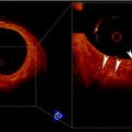
(or I), a (M + 1) × (N + 1) neighborhood $I\{i+m,j+n\}$ with $m\in \{-\frac{M}{2},\frac{M}{2}\}$ and $n\ \in \{-\frac{N}{2}, \frac{N}{2} \}$ calling sweeping window is being processed. Then, textural features are extracted from this sweeping window and assigned to the central pixel. Finally, according to the extracted features, pixels are classified into predetermined classes by the means of a classifier. It is worth mentioning that since IVUS images are circular cross section of the blood vessel, input images are converted into polar coordinates before applying texture analysis methods so that rectangular sweeping windows used for feature extraction are utilizable (Fig. 26.2).

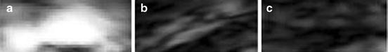
Fig. 26.1

Different tissue types in plaque area of IVUS images: (a) dense calcium, (b) necrotic core, and (c) fibro-lipid

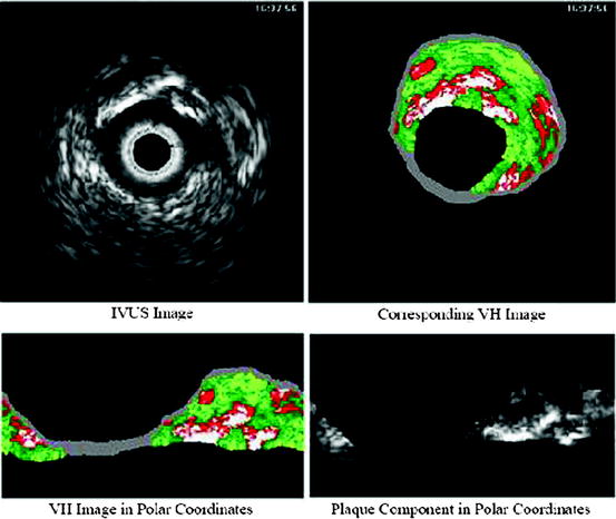
Fig. 26.2

Cartesian–Polar conversion of IVUS images for feature extraction

Figure 26.3 shows the outline of the project and the steps of Tissue Characterization stage. However, each of the proposed algorithms later explained in this chapter may follow some or all of these steps. It is worth defining the materials of these steps before stating the proposed algorithms.

Fig. 26.3

Outline of the project and steps of Tissue Characterization stage

Note: In this chapter, the plaque area is taken directly from the VH examples, in order for us to be able to validate the classification algorithms proposed here.

2 Materials and General Background

2.1 Feature Extraction Methods

Co-occurrence matrix and statistical properties:

A co-occurrence matrix, C, is used to describe the patterns of neighboring pixels in an image at a given distance d, and a given direction $\theta \in \left\{ {0^{\circ},45^{\circ},90^{\circ},135^{\circ}} \right\}$ corresponding to horizontal, diagonal, vertical, and anti-diagonal directions (Fig. 26.4). This matrix is somehow a second-order histogram of the image and gives information about the relative positions of the various gray levels within the image [1].

Fig. 26.4

The four directions used to form the co-occurrence matrix

Let us consider the neighborhood centered on the pixel (i, j) from image I. Its co-occurrence matrix is defined in a certain direction as ${C_{{d,\theta }}}(a,b)$ ,where $a,b\in [1,\ldots,P],$ where P refers to maximum gray level in image I and d is the gray level distance in the direction $\theta$ . Figure 26.5 gives a graphical description of this process for ${C_{{1,0^{\circ}}}}$ .

Fig. 26.5

Construction of the co-occurrence matrix in horizontal direction: (a) the original image, (b) horizontal neighboring of gray levels 1 and 4 with distance 1 occurred once in the image, and (c) the final result of the horizontal co-occurrence matrix

Various textural features can then be derived from co-occurrence matrix. For defining these textural features it is necessary to calculate the following statistical parameters in the first step:

${P^{{d,\theta }}}(a,b) = \frac{{{C_{{d,\theta (a,b)}}}}}{{\sum\limits_{a=1}^P {\sum\limits_{b=1}^P {{C_{{d,\theta (a,b)}}}} } }}$

(26.1)

$P_x^{{d,\theta }}(a)=\sum\limits_{b=1}^P {{P^{{d,\theta }}}(a,b)}$

(26.2)

$P_y^{{d,\theta }}(b)=\mathop{\sum}\limits_{a=1}^P{P^{{d,\theta }}}(a,b)$

(26.3)

$\begin{array}{lll} P_{x+y}^{{d,\theta }}(k)&=\mathop{\sum}\limits_{a=1}^P\mathop{\sum}\limits_{b=1}^P{P^{{d,\theta }}}(a,b),\quad a+b=k,\hfill\\ k&=2,\ldots,2P \end{array}$

(26.4)

$\begin{array}{lll} P_{x-y}^{{d,\theta }}(k)&=\mathop{\sum}\limits_{a=1}^P\mathop{\sum}\limits_{b=1}^P{P^{{d,\theta }}}(a,b),\quad \left| {a-b} \right|=k,\hfill\\ k&=1,\ldots,P-1 \end{array}$

(26.5)

$H{X^{{d,\theta }}}=-\mathop{\sum}\limits_{a=1}^PP_x^{{d,\theta }}(a)\log (P_x^{{d,\theta }}(a))$

(26.6)

$H{Y^{{d,\theta }}}=-\mathop{\sum}\limits_{b=1}^PP_y^{{d,\theta }}(b)\log (P_y^{{d,\theta }}(b))$

(26.7)

$HXY_1^{{d,\theta }}=-\mathop{\sum}\limits_{a=1}^P\mathop{\sum}\limits_{b=1}^P{P^{{d,\theta }}}(a,b)\log (P_x^{{d,\theta }}(a)P_y^{{d,\theta }}(b))$

(26.8)

$HXY_2^{{d,\theta }}{\,=\,}-\mathop{\sum}\limits_{a=1}^P\mathop{\sum}\limits_{b=1}^P P_x^{{d,\theta }}(a)P_y^{{d,\theta }}(b)\log (P_x^{{d,\theta }}(a)P_y^{{d,\theta }}(b))$

(26.9)

${Q^{{d,\theta }}}(a,b)=\mathop{\sum}\limits_{k=1}^P\frac{{{P^{{d,\theta }}}(a,k){P^{{d,\theta }}}(b,k)}}{{P_x^{{d,\theta }}(a)P_y^{{d,\theta }}(b)}}$

(26.10)

Based on these statistical parameters, the 14 Haralick texture features are defined as follows:

Angular second moment (ASM): this feature is a measure of smoothness of the image. The less smooth the image is, the lower is the ASM.

$f_1^{{d,\theta }}=\mathop{\sum}\limits_{a=1}^P\mathop{\sum}\limits_{b=1}^P{P^{{d,\theta }}}(a,b)$

(26.11)

Contrast: This feature is a measure of local gray-level variations.

$f_2^{{d,\theta }}=\mathop{\sum}\limits_{k=0}^{P-1 }{k^2}p_{x-y}^{{d,\theta }}(k)$

(26.12)

Correlation:

$f_3^{{d,\theta }}=\frac{{\sum\limits_{a=1}^P {\sum\limits_{b=1}^P {ab{p^{{d,\theta }}}(a,b)-{\mu_{x\ }}{\mu_y}} } }}{{{\sigma_x}{\sigma_y}}}$

(26.13)

Variance:

$f_4^{{d,\theta }}=\mathop{\sum}\limits_{a=1}^P\mathop{\sum}\limits_{b=1}^P{{(a-\mu )}^2}{p^{{d,\theta }}}(a,b)$

(26.14)

Inverse difference moment:

$f_5^{{d,\theta }}=\mathop{\sum}\limits_{a=1}^P\mathop{\sum}\limits_{b=1}^P\frac{1}{{1+{(a-b)^2}}}{p^{{d,\theta }}}(a,b)$

(26.15)

Sum average:

$f_6^{{d,\theta }}=\mathop{\sum}\limits_{k=2}^{2P }kp_{x+y}^{{d,\theta }}(k)$

(26.16)

Sum variance:

$f_7^{{d,\theta }}=\mathop{\sum}\limits_{k=2}^{2P }(k-f_6^{{d,\theta }})p_{x+y}^{{d,\theta }}(k)$

(26.17)

Sum entropy:

$f_8^{{d,\theta }}=\mathop{\sum}\limits_{k=2}^{2P }p_{x+y}^{{d,\theta }}(k)\log (p_{x+y}^{{d,\theta }}(k))$

(26.18)

Difference variance:

$f_9^{{d,\theta }}=-\mathop{\sum}\limits_{k=1}^{P-1 }p_{x-y}^{{d,\theta }}(k)\log (p_{x-y}^{{d,\theta }}(k))$

(26.19)

10.

Difference variance:

$f_{10}^{{d,\theta }} = -\mathop{\sum}\limits_{k=1}^{P-1 }p_{x-y}^{{d,\theta }}(k)\log (p_{x-y}^{{d,\theta }}(k))$

(26.20)

11.

Entropy: This feature is a measure of randomness of the image and takes low values for smooth images.

$f_{11}^{{d,\theta }} = -\mathop{\sum}\limits_{a=1}^P\mathop{\sum}\limits_{b=1}^P{p^{{d,\theta }}}(a,b)\log ({p^{{d,\theta }}}(a,b))$

(26.21)

12.

Information measure:

$f_{12}^{{d,\theta }}=\frac{{{f_{11 }}-HXY_1^{{d,\theta }}}}{{ \max (H{X^{{d,\theta }}},H{Y^{{d,\theta }}})}}$

(26.22)

$f_{13}^{{d,\theta }}=\sqrt{{1-\mathrm{ex}{{\mathrm{p}}^{{-2(HXY_2^{{d,\theta }}-f_{11}^{{d,\theta }})}}}}}$

(26.23)

13.

Maximal correlation coefficient:

$f_{14}^{{d,\theta }}=\sqrt{{\operatorname{second}\operatorname{largest}\operatorname{eigenvalue}\operatorname{of}{Q^{{d,\theta }}}}}$

(26.24)

Local binary pattern (LBP):

LBP is a structure-related measure in which a binary number is allocated to the circularly symmetric neighborhoods of the center pixel of the window being processed and the histogram of the resulting binary patterns can be used as a discriminative feature for texture analysis [2, 3]. Actually, in this method N neighbors of the center pixel (i, j) on a circle of radius R with coordinates $\left( {-R\sin \frac{{\pi n}}{N},R\cos \frac{{\pi n}}{N}} \right)\ (n\in \left\{ {0,\ldots,N-1} \right\})$ are processed. Typical neighbor sets $$ (N,R) $$

are (8, 1), (16, 2), and (24, 3), as shown in Fig. 26.6.

Fig. 26.6

Typical LBP binary patterns [4]

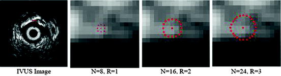
Fig. 26.7

Illustration of LBP, Left: the basic steps in computing the LBP code for a given pixel position: (a) the operator is centered on the given pixel and equidistant samples are taken on the circle of radius around the center; (b) the obtained samples are turned into 0’s and 1’s by applying a sign function with the center pixel value as threshold; (c) rotation invariance is achieved by bitwise shifting the binary pattern clockwise until the lowest binary number is found. Right: some of the microstructures that LBP are measuring [5]

As these coordinates do not match the coordinates of the processing window, their corresponding gray levels are estimated by interpolation. Let ${g_c}$ correspond to the gray value of the center pixel and ${g_n}$ correspond to the gray values of the N neighbor pixels. A binary digit is then allocated to each neighbor based on the following function:

$s({g_n}-{g_c})=\left\{ {\begin{array}{*{20}{c}} {1,{g_n}-{g_c}\geq 0} \\ {0,{g_n}-{g_c}<0} \\ \end{array}} \right.$

(26.25)

Then, by rotating the neighbor set clockwise the least significant resulting binary string is assigned to the processing as its binary pattern ${L_{R,N }}=\{L_{R,N}^0,\ldots,L_{R,N}^{N-1}\}$ . This way the local binary pattern is rotation invariant. The basic steps for calculating ${L_{R,N }}$ and some microstructures that binary patterns can detect in images are illustrated in Fig. 26.7.

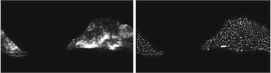
Based on the binary pattern ${L_{R,N }}$ and the gray values of neighbor pixels ${g_n},$ three texture features are defined as follows (Figs. 26.8, 26.9, and 26.10):

Fig. 26.8

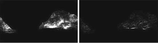
Illustration of $f_{R,N}^1$ feature for P = 8, R = 1: plaque area in polar coordinates (left) and $f_{R,N}^1$ (right)

Fig. 26.9

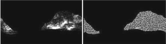
Illustration of $f_{R,N}^2$ feature for P = 8; R = 1: plaque area in polar coordinates (left) and $f_{R,N}^2$ (right)

Fig. 26.10

Illustration of $f_{R,N}^3$ feature for P = 8; R = 1: plaque area in polar coordinates (left) and $f_{R,N}^3$ (right)

$f_{R,N}^1=\mathop{\sum}\limits_{n=0}^{N-1 }L_{R,N}^n{2^n}$

(26.26)

$f_{R,N}^2=\mathrm{var}\{{g_n}\}$

(26.27)

$f_{R,N}^3=\left\{ {\begin{array}{*{20}{c}} {\mathop{\sum}\limits_{n=0}^{N-1 }L_{R,N}^n,} & {\ U({L_{R,N }})\leq 0} \\ {N+1,} & {\ \mathrm{otherwise}} \\ \end{array}} \right.$

(26.28)

Function U is a transition counter that counts the transition between 0 and 1 and vice versa in the binary pattern.

Run-length matrix:

One of the methods that has been extensively used in segmentation and texture analysis is run-length transform [1]. A gray-level run is a set of consecutive pixels having the same gray-level value. The length of the run is the number of pixels in the run. Run-length features encode textural information related to the number of times each gray-level appears in the image by itself, the number of times it appears in pairs, and so on. Let us consider the neighborhood centered on the pixel (i, j) from image I. Its run-length matrix is defined in a certain direction as ${R_k}(a,\ b),$ where $a\in \left[ {1,\ldots,P} \right],$ where P is maximum gray level and b is the run length, i.e., the number of consecutive pixels along a direction having the same gray-level value. In this approach each neighborhood is characterized with two run-length matrices: ${R_v}(a,\ b)$ and ${R_h}(a,\ b)$ corresponding to vertical and horizontal directions, respectively. Figure 26.11 shows the formation of run-length matrix.

Fig. 26.11

Run-length matrix (in horizontal direction) formation: (a) original intensity matrix and (b) run-length matrix

Let R be the maximum run-length, N _r be the total number of runs, and ${N_{\mathrm{p}}}$ be the number of pixels in the processing window. Run-length features are then defined as follows:

Galloway (traditional) run-length features: the five original features of run-length statistics derived by Galloway [6] are as follows:

Short run emphasis (SRE) (Fig. 26.12):

$f_1^k=\frac{1}{{{N_{\tau }}}}\mathop{\sum}\limits_{a=1}^P\mathop{\sum}\limits_{b=1}^R\frac{{{R_{k(a,b) }}}}{{{b^2}}}$

(26.29)

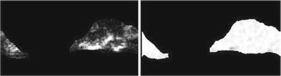
Fig. 26.12

Illustration of feature SRE: plaque area in polar coordinates (left) and SRE (right)
Long run emphasis (LRE) (Fig. 26.13):

$f_2^k = \frac{1}{{{N_{\tau }}}}\mathop{\sum}\limits_{a=1}^P\mathop{\sum}\limits_{b=1}^R{R_k}(a,b)\cdot {b^2}$

(26.30)

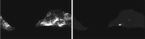
Fig. 26.13

Illustration of feature LRE: plaque area in polar coordinates (left) and LRE (right)
Gray-level nonuniformity (GLN) (Fig. 26.14):

$f_3^k=\frac{1}{{{N_{\tau }}}}\mathop{\sum}\limits_{a=1}^P{{\left( {\mathop{\sum}\limits_{b=1}^R{R_k}(a,b)} \right)}^2}$

(26.31)

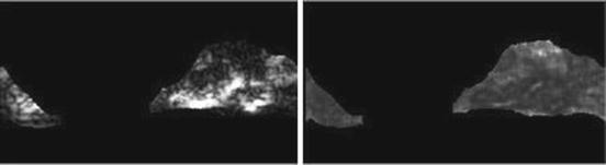
Fig. 26.14

Illustration of feature GLN: plaque area in polar coordinates (left) and GLN (right)
Run-length nonuniformity (RLN) (Fig. 26.15):

$f_4^k = \frac{1}{{{N_{\tau }}}}\mathop{\sum}\limits_{b=1}^R{{\left( {\mathop{\sum}\limits_{a=1}^P{R_k}(a,b)} \right)}^2}$

(26.32)

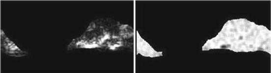
Fig. 26.15

Illustration of feature RLN: plaque area in polar coordinates (left) and RLN (right)
Run percentage (Fig. 26.16):

$f_5^k=\frac{{{N_{\tau }}}}{{{N_p}}}$

(26.33)

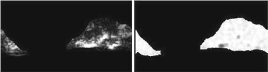
Fig. 26.16

Illustration of feature run percentage: plaque area in polar coordinates (left) and run percentage (right)

Chu run-length features: the following features proposed by Chu et al. extract gray-level information in run-length matrix:

Low gray-level run emphasis (LGRE) (Fig. 26.17):

$f_6^k=\frac{1}{{{N_{\tau }}}}\mathop{\sum}\limits_{a=1}^P\mathop{\sum}\limits_{b=1}^R\frac{{{R_k}(a,b)}}{{{a^2}}}$

(26.34)

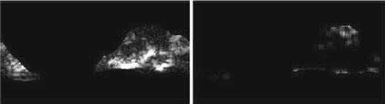
Fig. 26.17

Illustration of feature LGRE: plaque area in polar coordinates (left) and LGRE (right)

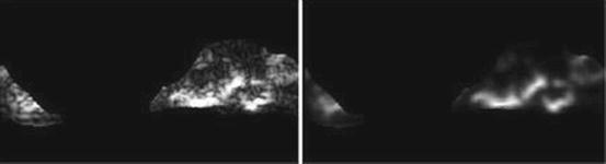
Fig. 26.18

Illustration of feature HGRE: plaque area in polar coordinates (left) and HGRE (right)
High gray-level run emphasis (HGRE) (Fig. 26.18):

$f_7^k = \frac{1}{{{N_{\tau }}}}\mathop{\sum}\limits_{a=1}^P\mathop{\sum}\limits_{b=1}^R{R_{{k(a,b)\cdot {a^2}}}}$

(26.35)

Dasarathy and holder features: these features follow the idea of joint statistical measure of gray level and run length:

Short run low gray-level emphasis (SRLGE) (Fig. 26.19):

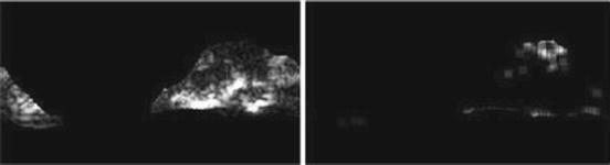
Fig. 26.19

Illustration of feature SRLGE: plaque area in polar coordinates (left) and SRLGE (right)

$f_8^k=\frac{1}{{{N_{\tau }}}}\mathop{\sum}\limits_{a=1}^P\mathop{\sum}\limits_{b=1}^R\frac{{{R_k}(a,b)}}{{{a^2}\cdot {b^2}}}$

(26.36)
Short run high gray-level emphasis (SRHGE) (Fig. 26.20):

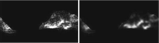
Fig. 26.20

Illustration of feature SRHGE: plaque area in polar coordinates (left) and SRHGE (right)

$f_9^k=\frac{1}{{{N_{\tau }}}}\mathop{\sum}\limits_{a=1}^P\mathop{\sum}\limits_{b=1}^R\frac{{{R_{{k(a,b)\cdot {a^2}}}}}}{{{b^2}}}$

(26.37)
Long run low gray-level emphasis (LRLGE) (Fig. 26.21):

Fig. 26.21

Illustration of feature LRLGE: plaque area in polar coordinates (left) and LRLGE (right)

$f_{10}^k = \frac{1}{{{N_{\tau }}}}\mathop{\sum}\limits_{a=1}^P\mathop{\sum}\limits_{b=1}^R\frac{{{R_k}(a,b)\cdot {b^2}}}{{{a^2}}}$

(26.38)
Long run high gray-level emphasis (LRHGE) (Fig. 26.22):

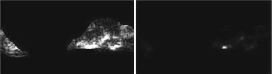
Fig. 26.22

Illustration of feature LRLGE: plaque area in polar coordinates (left) and LRHGE (right)

$f_{11}^k=\frac{1}{{{N_{\tau }}}}\mathop{\sum}\limits_{a=1}^P\mathop{\sum}\limits_{b=1}^R{R_{k(a,b) }}\cdot {a^2}\cdot {b^2}$

(26.39)

Above-mentioned methods have been previously used by several groups for IVUS plaque characterization. In next sections the proposed methods are introduced and discussed.

2.2 Feature Reduction

Linear discriminant analysis (LDA):

LDA are methods which are used in statistics and machine learning to find the linear combination of features which best separate two or more classes of objects or events. The resulting combination may be used as a linear classifier or, more commonly, for dimensionality reduction before later classification. Suppose that the feature vectors come from C different classes (each class with mean ${\mu_i}$ and covariance $\mathrm{Co}{{\mathrm{v}}_i}$ ), then the between class and within class scatter matrices are defined as follows:

${S_{\mathrm{b}}}=\frac{1}{c\ }\ \mathop{\sum}\limits_{i=1}^c({\mu_i}-\mu ){{(\mu -\mu )}^{\mathrm{T}}},\quad \mu =\frac{1}{c}\ \mathop{\sum}\limits_{i=1}^c({\mu_i})$

(26.40)

${S_{\mathrm{w}}}=\mathop{\sum}\limits_{i=1}^c\mathrm{Co}{{\mathrm{v}}_{i\ }}$

(26.41)

It is proved that eigenvectors of $S_{\mathrm{w}}^{-1 }{S_{\mathrm{b}}}$ are the directions that best separate these classes from each other [7]. Projecting feature vectors to the L (L < # of features) largest eigenvectors results in a new reduced feature vector that better suited to classification methods. Figure 26.23 shows a Fisher direction for a three class problem.

Fig. 26.23

Distribution of three classes and the Fisher direction that best separates these classes from each other

2.3 Classification

2.3.1 SVM Classifier

Support vector machines (SVM) are the classifiers based on the concept of decision planes that define decision boundaries. A decision plane is one that separates between a set of objects having different class memberships. A schematic example is shown in the illustration below. In this example, the objects belong either to class Black or White. The separating line defines a boundary on the right side of which all objects are Black and to the left of which all objects are White. The above is a classic example of a linear classifier, i.e., a classifier that separates a set of objects into their respective groups (Black and White in this case) with a line. Most classification tasks, however, are not that simple, and often more complex structures are needed in order to make an optimal separation, i.e., correctly classify new objects (test cases) on the basis of the examples that are available (train cases). Classification tasks based on drawing separating lines to distinguish between objects of different class memberships are known as hyperplane classifiers. Support vector machines are particularly suited to handle such tasks. Support vector machine (SVM) is primarily a classifier method that performs classification tasks by constructing hyperplanes in a multidimensional space that separates cases of different class labels. To construct an optimal hyperplane, SVM employs an iterative training algorithm which is used to minimize an error function. According to the form of the error function, SVM models can be classified into different distinct groups. The C-SVM type is used in all proposed algorithms. In a two-class case, if the training dataset consists of feature vectors $\{{f_1},\ldots,{f_n}\}$ with class labels ${y_i}\in \{-1,\ 1\}$ , then the SVM training problem is equivalent to finding W and b such that training involves the minimization of the error function [8] and [9]:

$\frac{{{W^{\mathrm{T}}}W}}{2}+C\sum\limits_{i=1}^N {{\zeta_i}}$

(26.42)

subject to the constraints:

$\begin{gathered}{y_i}({W^{\mathrm{T}}}\varphi ({x_i})+b)\geq 1-{\zeta_i}\;\mathrm{and}\;{\zeta_i}\geq 0, \quad i=1,\ldots, N\hfill\\ \end{gathered}$

(26.43)

where ${\zeta_i}\geq 0$ are the so-called slack variables that allow for misclassification of noisy data points, and parameter C > 0 controls the trade-off between the slack variable penalty and the margin [8]. In fact, W and b are chosen in a way that maximize the margin, or distance between the parallel hyperplanes that are as far apart as possible while still separating the data (Fig. 26.24). The function $\varphi (x)$ maps the data to a higher dimensional space. This new space is defined by its kernel function:

$K({f_i},{f_j})=\varphi {{({f_i})}^{\mathrm{T}}}\varphi ({f_j})$

(26.44)

The above problem can be formulated as a quadratic optimization process. The details of the solution and its implementation can be found in [10]. The Gaussian Radial Basis Function (RBF) kernel was used:

$K({f_i},{f_j})={{\mathrm{e}}^{{-\gamma \parallel {f_i}-{f_j}{\parallel^2}}}}$

(26.45)

This was firstly due to the fact that RBF kernel has only one parameter $\left( \gamma \right)$ to adjust. Also, SVM classifiers based on RBF kernel were found more accurate than linear, sigmoid, and polynomial kernels in case of our problem. The publicly available C++ implementation of the SVM algorithms known as LIBSVM [10] was used. The entire dataset was normalized prior to training by setting the maximum value of each feature to 1 and the minimum to 0. For each set of parameters, fivefold cross validation was performed: the SVM was trained using 80% of the data samples, classified the remaining 20%, and repeated the procedure for all five portions of the data (Fig. 26.25).

Fig. 26.24

Maximum-margin hyperplane and margins for a SVM trained with samples from two classes. Samples on the margin are called the support distribution

2.4 Post-processing

Studying intensity variety of each plaque component in VH images of the dataset through histogram analysis reveals that useful information can be extracted via this simple analysis. Figure 26.26 illustrates the histogram of pixels for three different plaque components. As this gray-scale-derived information might be ignored among many textural features in the classification steps, another step is added to the algorithm after the classification by SVM. In this step the given label of a pixel by SVM is confirmed or altered based on some prior information derived from the histogram of the IVUS image. Some useful information is pointed out below that can be inferred from the histograms displayed in Fig. 26.26:

Fig. 26.25

Example of misclassification that shows slack variables

Fig. 26.26

The histogram of pixels belonging to FF, DC, and NC classes for 400 out of 500 IVUS images

The majority of samples belong to FF class; however, there are few FF pixels whose their intensities exceed the gray level 150 (ThFF = 150).
Most of the pixels with intensities above the gray level 200 [ThDC (low) = 200] belong to the DC class, whereby few pixels with value under 50 [ThDC (high) = 50] belong to this class.
Pixels belonging to the NC are concentrated more between 30 and 200 gray levels [ThNC (low) = 30] and [ThNC (high) = 200].

So, based on these additional thresholds, the system will decide on whether to change the decision of SVM classifier or not.

2.5 Dataset

The data were acquired from 10 patients, which included about 2,263 gray-scale IVUS images and their corresponding VH images. These IVUS images of size 400 × 400 pixels were acquired using an electronic probe (In-Vision Gold, Volcano Therapeutics, Inc.) with a synthetic aperture 2.9 F and a frequency of 20 MHz. A motorized pullback was performed along the entire vessel with a speed of 1.0 mm/s using a dedicated pullback device. A total number of 500 frames from 12 vessels [6 left anterior descending (LAD), 3 right coronary artery (RCA), 3 left circumflex (LCX)] of 10 patients were available for VH analysis and comparison with IBH. In the VH analysis the total average amount of fibrous/fibro-fatty, dense calcium, and necrotic core was (1,505,907 pixels) 37,647 mm², (388,073 pixels) 9,701 mm², and (516,711 pixels) 12,917 mm², respectively. The relative average amounts per cross section were 63%, 16%, and 21%.

2.6 Statistical Analysis

The measures of sensitivity, specificity, and predictive accuracy for the three plaque components were calculated and reported as statistical analysis in this thesis. The standard formulae for these measures were the same commonly accepted in the medical literature [11].

$\mathrm{Sensitivity}=\frac{\mathrm{True}\ \mathrm{Positive}\ \mathrm{Decisions}}{\mathrm{Decisions}\ \mathrm{Actually}\ \mathrm{Positive}\ }$

(26.46)

$\mathrm{Specificity}=\frac{\mathrm{True}\ \mathrm{Negative}\ \mathrm{Decisions}}{\mathrm{Decisions}\ \mathrm{Actually}\ \mathrm{Negative}}$

(26.47)

$\mathrm{Accuracy}=\frac{\mathrm{All}\ \mathrm{Correct}\ \mathrm{Decisions}}{\mathrm{Total}\ \mathrm{Cases}}$

(26.48)

$\mathrm{C}{{\mathrm{I}}_{{0.95\%}}}=X \pm 1.96\times \frac{{X\times (1-X)}}{N}$

(26.49)

where

is either the sensitivity or specificity and $$ N $$

is the number of decisions used in denominator for calculating the sensitivity or specificity. In addition to the above-mentioned measures, Cohen’s Kappa index is calculated to quantify the degree of agreement between the Algorithm IV and VH classification for in vivo validation, and Algorithm IV and manual painted images for ex vivo validations. A kappa value of 0.41–0.60 indicates moderate (fair) agreement, 0.61–0.80 indicates good agreement, and 0.81–1.0 indicates excellent agreement. This metric was originally introduced by Cohen to determine the level of agreement between two observers [11]. The kappa is calculated as

$\kappa =\frac{{{\rho_o}-{\rho_c}}}{{1-{\rho_c}}}$

(26.50)

where ${\rho_o}$ is the observed proportion of agreement and ${\rho_c}$ is the expected proportion of agreement resulting from chance.

3 Algorithm I

3.1 Textural Feature Extraction

As it was mentioned in the previous section, various textural features can be derived from run-length matrix such as the short run emphasis, the long run emphasis, the gray-level nonuniformity, the run-length nonuniformity, and the run percentage. These features have been previously used on IVUS images; however, the results were not fulfilling [12]. Hence, two new features are proposed characterizing each gray-level a (i.e., every row) of the run-length matrix. The first feature $f_1^k(a),\quad k\in \{h,v\}$ where h and v represent horizontal and vertical respectively is defined as the maximum number of occurrences multiplied by the length of the run with maximum occurrence ${b_{\mathrm{m}}}$ :

$f_1^k(a)={R_k}(a,{b_{\mathrm{m}}})\times {b_{\mathrm{m}}},{b_{\mathrm{m}}}=\mathrm{ar}{{\mathrm{g}}_b}\ \max ({R_k}(a,b))$

(26.51)

And the second feature $f_1^k(a),\quad k\in \{h,r\}$ is defined as the sum of every occurrences multiplied by its corresponding run length:

$f_2^k(a)=\mathop{\sum}\limits_bb\times R(a,b)$

(26.52)

This way, each pixel (i, j) is mapped to a feature matrix, j:

${F_{i,j }}=\left( {\begin{array}{*{20}{c}} {f_1^h(1)} & {f_2^h(1)} & {f_1^v(1)} \\ {\begin{array}{*{20}{c}} \vdots \\ {f_1^h(a)} \\ \end{array}} & {\begin{array}{*{20}{c}} \vdots \\ {f_2^h(a)} \\ \end{array}} & {\begin{array}{*{20}{c}} \vdots \\ {f_1^v(a)} \\ \end{array}} \\ {\begin{array}{*{20}{c}} \vdots \\ {f_1^h(P)} \\ \end{array}} & {\begin{array}{*{20}{c}} \vdots \\ {f_2^h(P)} \\ \end{array}} & {\begin{array}{*{20}{c}} \vdots \\ {f_1^v(P)} \\ \end{array}} \\ \end{array}\begin{array}{*{20}{c}} {\ f_2^h(1)} \\ {\begin{array}{*{20}{c}} \vdots \\ {\ f_2^h(a)} \\ \end{array}} \\ {\begin{array}{*{20}{c}} \vdots \\ {\ f_2^h(P)} \\ \end{array}} \\ \end{array}} \right)$

(26.53)

Let us consider now each column ${F_{i,j,c }}$ of matrix ${F_{i,j }}$ as a signal that is a function of the gray level $$ a $$

. As shown in Fig. 26.27, these signals reveal different frequency contents. This motivates us to extract discriminative features from spatial-frequency representation of the signals. Therefore, each signal is decomposed into a detail $F_{i,j,c}^d$ and an approximation $F_{i,j,c}^a$ by means of $1\mathrm{D}$ discrete wavelet transform (DWT):

Fig. 26.27

Distribution of 5,000 bundle feature vectors for each plaque type. Top to down: DC, fibro lipid, and NC. Left to right: $f_1^h\operatorname{and}f_2^h$

$F_{i,j,c}^a[u]=({F_{i,j }}*l)[u]$

(26.54)

$F_{i,j,c}^d[u]=({F_{i,j }}*h)[u]$

(26.55)

Then, each DWT component $((F_{i,j,c}^a[u])\;\mathrm{and}\;(F_{i,j,c}^d[u]))$ is characterized by a set of statistical features, namely, its weighted mean, weighted variance, maximum of signal, and its index:

$\rho_{1,c}^k=\frac{1}{P}\mathop{\sum}\limits_{u=1}^Pu\times F_{i,j,c}^k(u)$

(26.56)

$\rho_{2,c}^k=\frac{1}{P}\mathop{\sum}\limits_{u=1}^P{{(u\times F_{i,j,c}^k(u)-\rho_{1,c}^k)}^2}$

(26.57)

$\rho_{3,c}^k=\max F_{i,j,c}^k(u)$

(26.58)

$\rho_{3,c}^k=\mathrm{ar}{{\mathrm{g}}_u}\max F_{i,j,c}^k(u)$

(26.59)

Furthermore, spectral behavior of these components is also characterized by means of autoregressive (AR) model of order 5:

$F_{i,j,c}^k(u)=\mathop{\sum}\limits_{t=1}^5F_{i,j,c}^k(u-t)\times \varphi_{t,c}^k+n(u)$

(26.60)

where

is the white noise and $\varphi_{t, c}^k$ are the coefficients of the AR model. These coefficients are also used as features.

Finally, the feature vector of each pixel $(i,\ j)$ is defined as follows:

$\begin{array}{lll} {X_{i,j }} &= \{\rho_{l,c}^k,\varphi_{t,c}^k,l\in \{1,\ldots,4\},t\in \{1,\ldots,5\}, \hfill\\ & \qquad c\in \{1,\ldots,4\},k\in \{a,d\}\} \end{array}$

(26.61)

This vector is the input of the SVM classifier. This classifier was explained in the classification subsection previously.

The block diagram of the proposed algorithm is shown in Fig. 26.28.

Fig. 26.28

Block diagram of the newly proposed modified run-length method

3.2 Result and Discussion of Algorithm I

The three feature extraction mentioned methods were then applied on the set of 200 frames. The characterized IVUS images were validated by their corresponding VH images and the accuracy, sensitivity, and specificity parameters were calculated for each technique. The results for this approach were compared to methods using LBP or co-occurrence-based features. The size of the neighborhood was empirically chosen to be 11 × 11 for all methods. This was done to get the optimum results for every method separately. For LBP method, five circles were then constructed in each neighborhood. Then, three features were extracted from each circle, and the number of features for every pixel in LBP method thus sums up to 15. Extracting features from five circles with different radii can be thought of as a multi-resolution textural analysis. Total number of features in the co-occurrence method was 14 which include, e.g., homogeneity, contrast, inverse difference moment, and so on. Results using different methods are presented below in Table 26.1. According to the results, Algorithm I is more capable of classifying DC and NC plaques in comparison to LBP or co-occurrence methods.

Table 26.1

The results of Algorithm I versus other techniques

	DC		FF		NC
Method	Sensitivity (%)	Specificity (%)	Sensitivity (%)	Specificity (%)	Sensitivity (%)	Specificity (%)	Overall accuracy (%)
LBP	45	96	97	42	30	95	71
Co-occurrence	67	95	84	80	53	83	75
Proposed method	70	95	84	75	55	82	77

Although this approach reveals a higher overall accuracy, the co-occurrence and LBP methods perform better in characterizing the fibro-lipid regions. Figure 26.29 illustrates the images characterized by all methods with their corresponding IVUS and VH images.

Fig. 26.29

The result of the feature extraction method in comparison with the co-occurrence and LBP methods from left to right (white is DC, green is fibro-lipid, and red is NC) (Color figure online)

In this study, the sensitivity of all methods for the detection of NC was low (55%). This fact was caused by similarities between NC and DC in gray-level IVUS images [13]. Furthermore, previous studies have shown that plaque areas adjacent to DC are frequently coded as NC tissue in VH images [14]. For a typical frame the proposed method took approximately 12 s to characterize the pixels, whereas the LBP took 2.6 min and the co-occurrence took nearly 60 min. Thus, in terms of time efficiency, the proposed method further outdoes the other two. A MATLAB implementation on an Intel Core 2 CPU2.00 GHz computer with 2.0 GB RAM was used in this work.

4 Algorithm II

For proposing this algorithm, this fact was taken into account that since each tissue shows different echogenic characteristics, the different plaque components can be characterized by their local frequency components. The best tool for this purpose is wavelet transform (WT). WT provides the best approximation of a space-frequency representation of an image, i.e., it permits to know which spectral components exist at which position in the input image. The main drawback of the WT is that it is translation non-invariant due to the decimation applied to the image after each decomposition level. Recently, another type of wavelet transforms known as redundant wavelet transforms (RWT) has been introduced [15]. Contrary to the classical WT, there is no decimation step after filtering the input image. This provides the decomposition to be translation invariant, and since it preserves the size of images in each level of decomposition, the local spectral components can be retrieved without any interpolation step. To generalize such transform, the wavelet packet transform (WPT) [16] has been introduced to decompose the whole-frequency spectrum into multiple sub-bands of varying sizes. It has been shown to provide a more redundant representation for the analysis of complex textural information. By combining the RWT and WPT, image can be decomposed into multiple sub-band images (Fig. 26.30). This decomposition provides translation invariance in addition to the rotation invariance gained by the initial polar transform.