and Dorin Comaniciu1
(1)
Imaging and Computer Vision, Siemens Corporate Technology, Princeton, NJ, USA
Abstract
In this chapter, we present an automatic object detection and segmentation framework based on Marginal Space Learning (MSL), which integrates the components described in previous chapters into a complete segmentation system. In addition, simple and efficient methods based on mesh resampling are developed to establish mesh point correspondence, required to train a mean shape for shape initialization and build a statistical shape model for object boundary delineation. We use the four-chamber heart segmentation in cardiac Computed Tomography (CT) data as an example to illustrate the segmentation framework. Most of the technologies developed for heart chamber segmentation are generic, therefore can be applied directly or adapted easily to segment other anatomies in different imaging modalities.
7.1 Introduction
Marginal Space Learning (MSL) is an effective tool to detect the pose of an anatomical structure in medical imaging. Examples of such applications are: detecting the brain mid-sagittal plane [41] or the spinal intervertebral disks [27, 28] for automatic alignment of MRI slice stacks, detecting the bounding box of the left ventricle in 2D MRI images [57], and detecting standard cardiac planes in 3D echocardiographic data [34]. In all the above applications, we only want to estimate the position, orientation, and scale of the target anatomical structures. However, in many other applications, the goal is segmenting the target anatomical structure from the surrounding tissues. Detailed and accurate boundary delineation is required. In this scenario, after detecting the pose with MSL, we align a mean shape with respect to the estimated position, orientation, and scale. If applicable, a few nonrigid deformation parameters are also estimated using nonrigid MSL [53]. Such aligned mean shape provides an initial estimate of the true shape and will be further refined during the subsequent boundary evolution.
In this chapter, we discuss an automatic object detection and segmentation framework based on the MSL. Its training procedure is composed of the following steps:
1.
Build an anatomically accurate mesh model to represent the boundary of the target anatomy. If the shape is simple, use a closed mesh to enclose the whole structure. If the shape is complex (e.g., the right ventricle that has separate inflow and outflow tracts ), use a parts based model [56, 58, 59] (see Chap. 5).
2.
Build an annotation tool and annotate enough number of training volumes, at least 50 datasets to start with for 3D problems.
3.
Establish mesh point correspondence across volumes. For a few geometrically simple shapes (e.g., a tube, a parabola, and other rotation symmetric shapes), we will show two mesh resampling methods to establish mesh correspondence. For more complicated shapes, Minimum Description Length (MDL) based approaches [11] can be used. Note that such optimization based approaches are often too computationally expensive to be practical.
4.
5.
7.
Train the MSL pose detectors using the image data and the corresponding pose ground truth of the target anatomical structure (see Chap. 2).
8.
Train a machine learning based boundary detector .
The detection and segmentation process on unseen data is composed of the following major steps.
1.
Use the MSL to generate the best pose candidates. If the object exhibits large shape variability, nonrigid MSL may also be exploited to estimate a few nonrigid deformation parameters (see Chap. 2).
2.
Aggregate the best pose candidates into the final estimate. If it is a prior known that there is only one object instance in the data, a simple average of the top candidates provides a good estimate. If there may be multiple instances of the same object type in the data, clustering should be used to select the final detections [27, 28].
3.
Align the mean shape with respect to the estimated pose to get an initial shape.
4.
Adjust each mesh point along the mesh surface normal to the optimal position where the response of the boundary detector is the largest.
5.
Enforce the prior shape constraint by projecting the adjusted mesh into a shape subspace .
6.
Repeat steps 4 and 5 a few iterations to improve the segmentation accuracy.
The object detection and segmentation framework presented in this chapter integrate the components described in the previous chapters. We also present a few methods that are integral part of the segmentation framework, but only briefly mentioned in the previous chapters. For example, in Chap. 6, we presented an optimization based method to calculate the optimal mean shape from a training set. There, we assumed that the annotated meshes had intrinsic anatomical correspondence across volumes. The mesh resampling based methods presented in this chapter are exemplar techniques to establish mesh point correspondence , being simple and efficient. Another topic presented in this chapter covers the boundary delineation, built upon learning based boundary detectors and a statistical shape model .
We will use four-chamber heart segmentation in cardiac Computed Tomography (CT) data as an example to illustrate the segmentation framework. This was in fact one of the first applications of the MSL [51, 52]. Most of the technologies developed for heart chamber segmentation are generic, therefore can be directly applied or easily adapted to segment other anatomies in different imaging modalities. On the other hand, different applications may have different clinical requirements, demanding some adaptation. For example, in left ventricle endocardium segmentation, it is preferred to have a smooth mesh tightly enclosing the blood pool (i.e., including the papillary muscles and trabeculation in the endocardium mesh). We therefore developed a special mesh refinement process that improves the left ventricle endocardium segmentation accuracy to meet the clinical requirements.
The remainder of this chapter is organized as follows. In Sect. 7.2, we review the previous work on heart chamber modeling and segmentation. The four-chamber heart model is presented in Sect. 7.3. In this section, we also present two mesh resampling based methods to establish point correspondence and the statistical shape model to enforce shape constraint. The process of nonrigid deformation estimation for boundary delineation is described in details in Sect. 7.4. A special mesh refinement process is developed in Sect. 7.5 to search for an optimal smooth left ventricle endocardium mesh to tightly enclose the blood pool. Quantitative evaluation on a large dataset in Sect. 7.6 demonstrates the efficiency and accuracy of the MSL based heart chamber segmentation method. This chapter concludes with Sect. 7.7.
7.2 Related Work on Heart Modeling and Segmentation
This section provides a brief review of the previous work on heart modeling and segmentation.
7.2.1 Heart Modeling
Geometric heart modeling is not a trivial task since the heart is a complex nonrigid organ, with multiple moving parts. The model must be anatomically accurate, accept manual editing, and provide sufficient information to guide automatic detection and segmentation. Except for a four-chamber heart model from [14] and [31], most of the previous work was focused on the Left Ventricle (LV) and/or the Right Ventricle (RV) . A closed mesh was often used to represent heart chambers [18, 24, 33]. Nevertheless, it is not clear how the atria interacted with the ventricles around the mitral and tricuspid valves in [33]. The heart model in [31] was more accurate in anatomy and it also included trunks of the major vessels connected to heart chambers. However, artificial patches were added at all valves to close the chamber meshes. These artificial patches were not processed with a special care in the segmentation algorithm; therefore, they could not be delineated accurately [14]. In our heart model, we keep the mesh open at a valve. Mesh points at the valve rim are labeled as control points , being treated differently to the normal mesh points during automatic segmentation.
The statistical shape model [9] is used in nonrigid object segmentation to enforce shape constraints and to make the system more robust. However, to build a statistical shape model, it is necessary to establish point correspondence among a group of shapes [9]. There are a few papers on building a 3D statistical shape model automatically using pair-wise or group-wise registration based approaches [16, 32], which are time consuming. Another approach is to establish correspondence among shapes through mesh resampling . Although this is difficult for a generic 3D shape, we can consistently resample the surface to establish correspondence for a few simple shapes (e.g., a tube and a parabola) [19, 24].
7.2.2 Heart Segmentation
Given the heart model, the segmentation task is to fit the model onto an unseen volume. Since the heart is a nonrigid shape , the model fitting (or heart segmentation) procedure can be divided into two steps: object localization and boundary delineation. Most of the previous approaches were focused on boundary delineation using Active Shape Models (ASM) [2], Active Appearance Models (AAM) [1, 37], or deformable models [3, 10, 14, 20, 36, 40]. The above segmentation technologies suffer from two limitations: (1) Most of them are semi-automatic and proper manual initialization is demanded. (2) Gradient descending based search in some of the approaches are likely to converge to a sub-optimal solution .
Object localization, a task largely ignored by early work in heart segmentation, is required for an automatic segmentation system. The MSL computational framework for object detection and pose estimation thus fills an important gap in a 3D heart segmentation pipeline, by efficiently providing automatic detection of the heart parts, and estimating their 3D pose and initial mean shape.
7.3 Four-Chamber Heart Modeling
In this section, we describe our four-chamber heart model . As part of the model, some mesh points are special and correspond to distinctive anatomical structures, such as those around the valve annulus. We label these points as control points. They are integral part of the mesh model in the sense that they are also connected to other mesh points with mesh triangles.
7.3.1 Left Ventricle and Left Atrium Models
A closed mesh has been used to represent the Left Ventricle (LV) [18, 24, 33]. Due to the lack of object boundary on the image, it is hard to consistently delineate the interfaces among the LV main body, the Left Ventricular Outflow Tract (LVOT) , and the basal area around the mitral valve . The mesh often cuts the LVOT and the mitral valve at an arbitrary position [18, 24, 33]. In our heart model, the mitral valve is explicitly represented as a closed contour along its border. Since we exclude the moving valve leaflets (which are hardly visible) from the model, the basal area can be delineated more consistently. Both the endo- and epi-cardiums are delineated for the LV. The commissure contour of both surfaces corresponds to the mitral valve annulus on one side and the aortic valve annulus (lying at the bottom edge of the Valsalva sinuses ) on the other side, as shown in Fig. 7.2d. Three curves are formed by control points around the mitral valve, namely, the mitral lateral (16 points), the mitral septum (15 points), and the LVOT lateral (16 points). As shown in Fig. 7.1a, they define two closed regions, one for the interface between the LV and the Left Atrium (LA) , and the other for the LV and the LVOT. The aortic valve (annotated with 32 points) is approximated as a plane, which cuts the valve at the bottom of the Valsalva sinuses . The LA is represented as an open mesh with an open area enclosed by the mitral septum and the mitral lateral control points (as shown in Fig. 7.1b). Figure 7.2 shows the LV/LA meshes with the control points (dots that are connected appropriately to form contours in the figure). The LV endocardium , epicardium , and LA meshes are represented with 545 points and 1,056 triangles each. The LVOT mesh is represented with 64 points and 64 triangles.
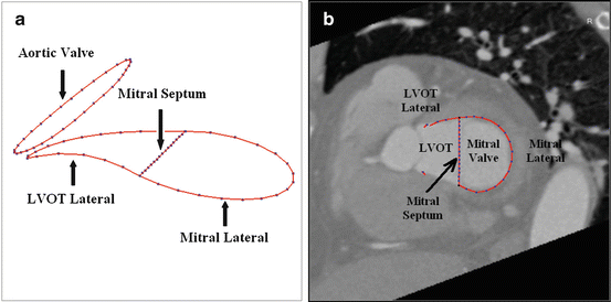
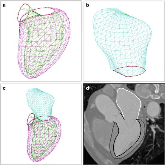

Fig. 7.1
Delineating the mitral and aortic valves. (a) A 3D view of the control points around the mitral and aortic valves. (b) Control points around the mitral valve embedded in a CT volume. Since the curves are 3D, they are only partially visible on a specific plane

Fig. 7.2
Left Ventricle (LV) and Left Atrium (LA) meshes. The control points are shown as dots and connected appropriately to form contours. (a) LV mesh. The inner mesh is endocardium; the outer mesh is epicardium; and Left Ventricular Outflow Tract (LVOT) is a short region connecting the aortic valve and mitral valve. (b) LA mesh. (c) Combined mesh of the LV and LA. (d) LV/LA meshes embedded in a CT volume
7.3.2 Right Ventricle and Right Atrium Models
The Right Ventricle (RV) has a complicated shape with separate inflow and outflow portions . Using a plane (indicated by a horizontal black line in Fig. 7.3a) passing the divergence point of the inflow and outflow tracts, we can naturally split the RV into three parts with the RV main body lying below the cutting plane. We call this plane “the RV divergence plane.” During the manual labeling of ground truth, the RV divergence plane is determined in the following way. We first determine the tricuspid valve , which is approximated as a plane. We then move the plane toward the RV apex to a position where the RV inflow and outflow tracts diverge. As shown in Fig. 7.3b, two curves, tricuspid lateral (23 points) and Right Ventricular Outflow Tract (RVOT) lateral (15 points), are annotated on the RV divergence plane to define the inflow and outflow connections. On a short axis view, the RV main body is a crescent (as shown in Fig. 7.3b and c). Two cusp points on the intersection are important landmarks, and an automatic detection algorithm is able to detect them reliably. They are explicitly represented in our model (Fig. 7.3d). The tricuspid (28 points) and pulmonary (18 points) valves are approximated as a plane. Similar to the LA, the Right Atrium (RA) is represented as an open mesh with the open area defined by the tricuspid valve. Figure 7.4 shows the RV/RA meshes with the control points (dots that are connected appropriately to form contours in the figure). In our model, the RV is represented with 761 points and 1,476 triangles and the RA is represented with 545 points and 1,056 triangles.
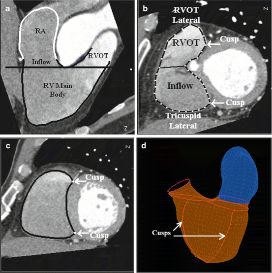
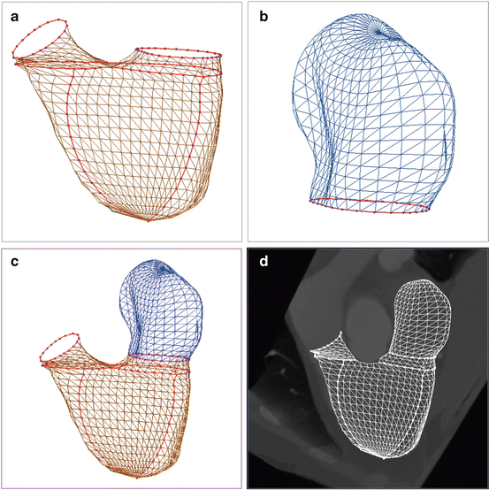

Fig. 7.3
Delineating the Right Ventricle (RV) control points. (a) The divergence plane (indicated by the horizontal line) of the RV inflow and outflow tracts splits the RV into three parts. (b) Delineating the divergence plane. (c) Inter-ventricular septum cusps labeled on a short-axis slice. (d) 3D visualization of the RV and Right Atrium (RA) meshes with inter-ventricular septum cusps indicated

Fig. 7.4
Right Ventricle (RV) and Right Atrium (RA) meshes. The control points are shown as dots and connected appropriately to form contours. (a) RV mesh. (b) RA mesh (c) Combined mesh of the RV and RA. (d) 3D visualization of the RV/RA meshes embedded in a CT volume
7.3.3 Establishing Point Correspondence
After object pose estimation, we use the aligned mean shape as an initial estimate of the true shape. To calculate the mean shape, we demand the annotated training meshes to have intrinsic anatomical correspondence across volumes. Furthermore, we use the Active Shape Model (ASM) to enforce the shape constraint during boundary evolution. To build the statistical shape model of the ASM, we also need the point correspondence . Establishing mesh point correspondence is a difficult task for a generic 3D shape. Fortunately, for a few simple shapes, such as a tube or a parabola, we can consistently resample the surface to establish this correspondence. Since it is much easier to consistently resample a 2D curve, we use a few planes to cut the 3D mesh to get a set of 2D intersection curves. The resulting 2D curves are uniformly sampled to get a point set with built-in correspondence. Using different methods to select cutting planes, we develop two resampling schemes, the rotation-axis based method for simple parabola-like shapes such as the LV , LA , and RA , and parallel-slice based method for the more complicated RV. In both methods, the long axis of a chamber needs to be determined from the annotated mesh. Generally, we define the long axis as the line connecting the center of a valve and the mesh point farthest from the valve (which often corresponds to the apex). For example, the LV long axis is the line connecting the mitral valve center and the LV apex . The RV long axis is determined as a line passing the RV apex and perpendicular to the divergence plane .
The rotation-axis based method is appropriate for a roughly rotation symmetric shape. Cutting the mesh with a plane passing the rotation axis, we get a 2D intersection. As shown in Fig. 7.5b, the rotation axis separates the intersection into two parts, which can be uniformly resampled independently. We then rotate the plane around the axis to get another intersection and resample the intersection in the same way. Repeating the above process, we achieve a set of points with built-in correspondence. We use this approach to resample the LV, LA, and RA, and also the LVOT , and RV inflow and outflow tracts , which can be approximated as tubes. To establish the correspondence between the cutting planes, we need a consistent way to determine the first cutting plane, which is often based on an anatomical landmark. Different chambers may use different landmarks. For the LV, we pick the cutting plane passing the aortic valve center as the first cutting plane.
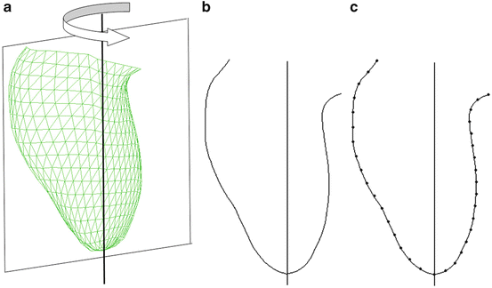

Fig. 7.5
The rotation-axis based resampling method demonstrated for the Left Ventricle (LV) endocardium mesh. (a) The LV endocardium mesh with its long axis. A cutting plane passing the long axis is also illustrated. (b) The intersection of the mesh with the cutting plane. (c) Resampled points indicated as dots. ©2008 IEEE. Reprinted, with permission, from Zheng, Y., Barbu, A., Georgescu, B., Scheuering, M., Comaniciu, D.: Four-chamber heart modeling and automatic segmentation for 3D cardiac CT volumes using marginal space learning and steerable features. IEEE Trans. Medical Imaging 27(11), 1668–1681 (2008)
The rotation-axis based method is not applicable to the RV main body since it is not rotation symmetric. Instead, a parallel-slice based method is developed for the RV, where we use a plane perpendicular to the RV long axis to cut the 3D mesh, as shown in Fig. 7.6a. The shape of an RV short-axis intersection is a crescent containing two cusp points (which have a high curvature and can be reliably determined from the intersection contour). They split the contour into two parts and each can be uniformly resampled, as shown in Fig. 7.6c.
Compared to other approaches [11, 16, 32] for establishing point correspondence, our solution is simple and each shape is processed independently. No time-consuming and error-prone 3D registration is necessary. Although our approach is not as generic as [11, 16, 32], it provides superior results for the heart chambers.


Fig. 7.6
The parallel-slice based resampling method for the Right Ventricle (RV) main body. (a) The RV main body mesh. A cutting plane perpendicular to the RV long axis is also illustrated. (b) The crescent-shaped intersection of the mesh with the cutting plane. Two cusps separate the intersection into two parts and each can be uniformly resampled independently. (c) Resampled points indicated as dots. ©2008 IEEE. Reprinted, with permission, from Zheng, Y., Barbu, A., Georgescu, B., Scheuering, M., Comaniciu, D.: Four-chamber heart modeling and automatic segmentation for 3D cardiac CT volumes using marginal space learning and steerable features. IEEE Trans. Medical Imaging 27(11), 1668–1681 (2008)
7.3.4 Statistical Shape Model
The statistical shape model [9] (a.k.a., the point distribution model ) is widely used in computer vision and medical image analysis to enforce prior shape constraint during the segmentation of a nonrigid object. The statistical shape model is learned from a set of training shapes,  . Each shape M i is composed of the same number of points J and can be represented as
  . Point
  is assumed to have correspondence across volumes. That means it represents the same anatomical position in different volumes. The point correspondence can be established by various methods, such as the mesh resampling techniques presented in the previous section.
 . Each shape M i is composed of the same number of points J and can be represented as
  . Point
  is assumed to have correspondence across volumes. That means it represents the same anatomical position in different volumes. The point correspondence can be established by various methods, such as the mesh resampling techniques presented in the previous section.
Before performing shape analysis , the external transformations of the training shapes need to be compensated. That means we need to transform the shapes to the same coordinate system. This process, called Generalized Procrustes Analysis (GPA) [13], searches for a mean shape  and an optimal transformation
  for each individual shape M i to minimize the sum of residual errors after alignment,

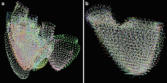
The similarity transformation is used as T in GPA and is often solved using an iterative approach. Please refer to Sect. 6.3.2 of Chap. 6 for an in-depth discussion on GPA. Figure 7.7 shows the RV shapes before and after the GPA.
 and an optimal transformation
  for each individual shape M i to minimize the sum of residual errors after alignment,
(7.1)

Fig. 7.7
Generalized Procrustes analysis of the right ventricle meshes (761 points). (a) Before alignment. (b) After alignment
Suppose after alignment a training shape M i is transferred to m i . The mean shape  over the whole training set after alignment is

The residual, d m i , of each shape to the mean shape is

The covariance matrix  , which is a 3J × 3J symmetric matrix, of the aligned shapes is calculated as

Using eigen-decomposition , the covariance matrix  can be decomposed as
![$$\displaystyle\begin{array}{rcl} \boldsymbol{\varPhi }& =& \mathbf{P}\varLambda {\mathbf{P}}^{T} \\ & =& [\mathbf{P}_{1},\mathbf{P}_{2},\ldots,\mathbf{P}_{3J}]diag(\lambda _{1},\lambda _{2},\ldots,\lambda _{3J}){[\mathbf{P}_{1},\mathbf{P}_{2},\ldots,\mathbf{P}_{3J}]}^{T},{}\end{array}$$](/wp-content/uploads/2016/08/A314110_1_En_7_Chapter_Equ5.gif)
where λ i is an eigenvalue and P i is the corresponding eigenvector. Since  is a real symmetric matrix that is semi-positive definite, all of its eigenvalues are non-negative real numbers. Without loss of generality, suppose the eigenvalues are ordered as
  . In the statistical shape model , the linear space represented by P is often called the shape space and each axis of the space, P i , is called a deformation mode . Its corresponding eigenvalue λ i is the amount of the variation of this deformation mode. The total variation λ T is

 over the whole training set after alignment is
(7.2)

(7.3)
 , which is a 3J × 3J symmetric matrix, of the aligned shapes is calculated as
(7.4)
 can be decomposed as
![$$\displaystyle\begin{array}{rcl} \boldsymbol{\varPhi }& =& \mathbf{P}\varLambda {\mathbf{P}}^{T} \\ & =& [\mathbf{P}_{1},\mathbf{P}_{2},\ldots,\mathbf{P}_{3J}]diag(\lambda _{1},\lambda _{2},\ldots,\lambda _{3J}){[\mathbf{P}_{1},\mathbf{P}_{2},\ldots,\mathbf{P}_{3J}]}^{T},{}\end{array}$$](/wp-content/uploads/2016/08/A314110_1_En_7_Chapter_Equ5.gif)
(7.5)
 is a real symmetric matrix that is semi-positive definite, all of its eigenvalues are non-negative real numbers. Without loss of generality, suppose the eigenvalues are ordered as
  . In the statistical shape model , the linear space represented by P is often called the shape space and each axis of the space, P i , is called a deformation mode . Its corresponding eigenvalue λ i is the amount of the variation of this deformation mode. The total variation λ T is
(7.6)
A shape in the training set can be presented as the mean shape plus a weighted sum of the deformation modes,

where  is a vector of weights. Since eigenvectors P i are orthonormal to each other, the weight w i can be easily calculated by the dot product of vectors m and P i ,

In general, a shape out of the training set cannot be represented exactly with Eq. (7.7). However, if the training set is large enough and can well represent the diversity of the whole shape population of the target object, the representation residual error is small.

(7.7)
 is a vector of weights. Since eigenvectors P i are orthonormal to each other, the weight w i can be easily calculated by the dot product of vectors m and P i ,
(7.8)
In practice, we do not want to use the full shape space learned from a training set. The first t deformation modes explain most amount of the shape variation and the remaining modes mainly correspond to noise in the data. Therefore, a shape m is often approximated as

This process is often called a projection into a shape subspace. The shape space is often truncated such that a certain amount α (e.g., α = 98 %) of variation is preserved. Therefore, t is the minimum integer such that

By varying the weights w i in Eq. (7.9), a new shape can be generated. To make the generated shape similar to those in the training set, we often enforce a limit to the weights,


(7.9)

(7.10)

(7.11)
The covariance matrix  in Eq. (7.4) has a dimension of 3J × 3J. In most of our applications, a shape is represented as a dense mesh to achieve a detailed segmentation of the object. For example, our whole heart model is represented as 3,005 points. The corresponding covariance matrix has a dimension of 9, 015 × 9, 015, which consumes a lot of memory (310 MB if the values are represented as 4-byte ‘double’ variables) and eigen-decomposition of such a huge matrix can be quite slow. Fortunately, the rank of the covariance matrix
  is bounded,

In practice, the number of training shapes, N, is much smaller than the number of points in a shape, therefore N < < 3J. For example, our heart chamber detectors are trained on no more than 500 volumes. That means most eigenvalues of  are zero. To enforce statistical shape constraint, the deformation modes with small (or zero) eigenvalues are discarded. It is not necessary to calculate those eigenvectors at all.
 in Eq. (7.4) has a dimension of 3J × 3J. In most of our applications, a shape is represented as a dense mesh to achieve a detailed segmentation of the object. For example, our whole heart model is represented as 3,005 points. The corresponding covariance matrix has a dimension of 9, 015 × 9, 015, which consumes a lot of memory (310 MB if the values are represented as 4-byte ‘double’ variables) and eigen-decomposition of such a huge matrix can be quite slow. Fortunately, the rank of the covariance matrix
  is bounded,
(7.12)
 are zero. To enforce statistical shape constraint, the deformation modes with small (or zero) eigenvalues are discarded. It is not necessary to calculate those eigenvectors at all.
In the following, we present two efficient methods to calculate the eigenvectors P i of  based on the fact that
  has a low rank. We can write the residual vectors of aligned training shapes d m i into a matrix,
![$$\displaystyle{ \mathbf{D} = [d\mathbf{m}_{1},d\mathbf{m}_{2},\ldots,d\mathbf{m}_{N}]. }$$](/wp-content/uploads/2016/08/A314110_1_En_7_Chapter_Equ13.gif)
The dimension of matrix D is 3J × N. We then perform Singular Value Decomposition (SVD) of matrix D directly, without calculating the covariance matrix  at all. Suppose matrix D can be decomposed as

where U is a 3J × 3J matrix;  is a 3J × N rectangular matrix with nonzero eigenvalues
  at the diagonal; and V is an N × N matrix. Here, U and V are orthonormal,
  and
and  . Then,
  can be represented as follows,
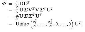
The above equation is an eigen-decomposition of  . The largest N eigenvalues λ i of
  is related to the eigenvalues σ i of D as

The remaining eigenvalues are zero. Eigenvector P i of  is a left-eigenvector of D, P i = U i . The SVD of D is much faster than eigen-decomposition of
  since matrix D has a lower dimension.
 based on the fact that
  has a low rank. We can write the residual vectors of aligned training shapes d m i into a matrix,
![$$\displaystyle{ \mathbf{D} = [d\mathbf{m}_{1},d\mathbf{m}_{2},\ldots,d\mathbf{m}_{N}]. }$$](/wp-content/uploads/2016/08/A314110_1_En_7_Chapter_Equ13.gif)
(7.13)
 at all. Suppose matrix D can be decomposed as
(7.14)
 is a 3J × N rectangular matrix with nonzero eigenvalues
  at the diagonal; and V is an N × N matrix. Here, U and V are orthonormal,
  and
and  . Then,
  can be represented as follows,
(7.15)
 . The largest N eigenvalues λ i of
  is related to the eigenvalues σ i of D as
(7.16)
 is a left-eigenvector of D, P i = U i . The SVD of D is much faster than eigen-decomposition of
  since matrix D has a lower dimension.
Alternatively, we can calculate another covariance matrix  as
as

The dimension of matrix  is N × N, which is much smaller than that of
  . Suppose the eigen-decomposition of
  is
is
![$$\displaystyle\begin{array}{rcl} \boldsymbol{\varPsi }& =& \mathbf{Q}\mathbf{S}{\mathbf{Q}}^{T} \\ & =& [\mathbf{Q}_{1},\mathbf{Q}_{2},\ldots,\mathbf{Q}_{N}]diag(s_{1},s_{2},\ldots,s_{N}){[\mathbf{Q}_{1},\mathbf{Q}_{2},\ldots,\mathbf{Q}_{N}]}^{T}.{}\end{array}$$](/wp-content/uploads/2016/08/A314110_1_En_7_Chapter_Equ18.gif)
That means

Left multiply both sides of the equation with D, we get

That means  has the same eigenvalues as
  , (s i = λ i ); and for an eigenvector Q i of
  , if we left multiple it with D, it is an eigenvector of
  , (P i = DQ i ).
 as
as
(7.17)
 is N × N, which is much smaller than that of
  . Suppose the eigen-decomposition of
  is
is![$$\displaystyle\begin{array}{rcl} \boldsymbol{\varPsi }& =& \mathbf{Q}\mathbf{S}{\mathbf{Q}}^{T} \\ & =& [\mathbf{Q}_{1},\mathbf{Q}_{2},\ldots,\mathbf{Q}_{N}]diag(s_{1},s_{2},\ldots,s_{N}){[\mathbf{Q}_{1},\mathbf{Q}_{2},\ldots,\mathbf{Q}_{N}]}^{T}.{}\end{array}$$](/wp-content/uploads/2016/08/A314110_1_En_7_Chapter_Equ18.gif)
(7.18)

(7.19)

(7.20)
 has the same eigenvalues as
  , (s i = λ i ); and for an eigenvector Q i of
  , if we left multiple it with D, it is an eigenvector of
  , (P i = DQ i ).
Both alternative methods presented here are much more efficient to calculate the eigenvalues and eigenvectors of  than working directly on
  . Among all three methods, the one based on the eigen-decomposition of the covariance matrix
  is the most efficient in our applications since
  has the smallest dimension of N × N when N < 3J.
 than working directly on
  . Among all three methods, the one based on the eigen-decomposition of the covariance matrix
  is the most efficient in our applications since
  has the smallest dimension of N × N when N < 3J.
7.4 Nonrigid Deformation Estimation for Heart Chambers
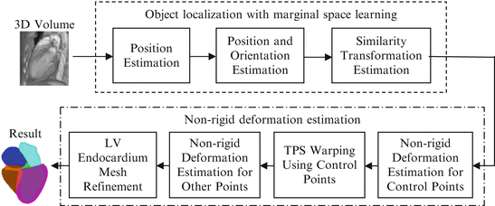
In this section, we present the MSL based heart chamber detection and segmentation method. The system diagram is shown in Fig. 7.8. We first automatically estimate the pose of heart chambers using the MSL and the mean shape is aligned with respect to the estimated pose to get an initial shape. The initial shape is further deformed to fit the object boundary under the guidance of a learning based boundary detector and a statistical shape model . Since the MSL based object pose estimation has been discussed in detail in the previous chapters, in the following we will skip this step. Instead, we focus this section on nonrigid deformation estimation .

