Fig. 12.1
The principle of fiber tracking . (a) Schematic view of a person watching a flower. Information is transported from the eye to the visual cortex at the back of the head. (b) Close-up of the voxel-wise diffusion measurement. The optical tract shows anisotropic (ellipsoid) water displacement and the tract can be reconstructed using diffusion tensor imaging
Figure 12.1b illustrates a straightforward approach to reconstruct tracts from the tensor ellipsoids , the so-called FACT algorithm (FACT = fiber assignment by continuous tracking ) [4, 5]. The tract is started in one voxel and it follows the orientation of the ellipsoid in this voxel until it hits the border of the voxel. Then, this process is iterated in the adjacent voxel. Usually several starting points—which are also called seeds —are chosen. For example, in Fig. 12.1b, the tract starting in the center of the initial voxel does not reach the end of the optic nerve tract, since the tract is interrupted when it reaches a voxel with isotropic diffusion. The other tract, which starts in the upper part of the initial voxel, reaches the visual brain cortex. Thus, by choosing several seeds instead of only one seed, the chance is increased that the actual tract is reconstructed.
In Fig. 12.1b, an important property of fiber tracking results can be appreciated: the strong dependency on the chosen algorithm and its parameters. The termination criterion of the algorithm depicted in Fig. 12.1b is to stop the tract if an isotropic voxel is reached. However, if the tract were allowed to maintain its direction in an isotropic voxel under the condition that the next voxel is anisotropic, then the broken fiber would make it to the end of the optic tract. In practice, of course, voxels are usually not perfectly isotropic, so one would rather choose a certain anisotropy threshold to terminate the fiber. The final tracking result will in any case depend strongly on this threshold. As there is often no unique and perfect choice of algorithm and parameters, the obtained results should not be regarded as a perfect ground truth. Nonetheless, it has been shown that the main fiber tracts can be reconstructed correctly.
Since the initial works on fiber tracking, many fiber tracking algorithms and strategies have been developed. Since a detailed review of these techniques is beyond the scope of this introduction and covered in Chap. 11 of this book, here we only present an in-depth description of the algorithm used for the fiber tracking in the “Three-Dimensional Tract Representation” section.
Protocol
Data Acquisition
The data were acquired using a 3 T scanner (TIM Trio, Siemens, Erlangen, Germany) equipped with a 32-channel head coil. A single-shot echo-planar imaging (EPI) sequence was applied for DTI assessment (TR 6400 ms, TE 91 ms, 96 × 96 matrix size, field of view 240 mm). Fifty axial slices with a thickness of 2.5 mm and no gap, 60 gradient directions, and two b-values (0 and 1000 s/mm2) were obtained.
Data Preprocessing
Eddy currents and head motion were corrected using FSL flirt (www.fmrib.ox.ac.uk/fsl/) by affine registration of the baseline and diffusion weighted volumes to the first baseline volume. Gradient directions were corrected according to the transformation. FSL bet was used in order to estimate brain masks. Tensors were fit using the teem library (teem.sourceforge.net). Negative Eigenvalues were corrected by adding (to all Eigenvalues) the amount by which the smallest is negative (corresponding to increasing the non-diffusion weighted image value).
Tracking Algorithm
The tractography algorithm that was used to generate the fiber tracking results was originally introduced by Reisert et al. [8] and is a so-called global tracking algorithm [9, 10]. This algorithm ranked first in an evaluation study by Fillard et.al. on the performance of tractography algorithms [11] and is implemented in MITK-Diffusion ([12], www.mitk.org/Difu sion). The complete procedure is described in more detail in [13].
Two-Dimensional Tract Representation
Introduction (2D)
Here we present a diffusion tensor imaging derived color map produced using MITK-Diffusion ([12], www.mitk.org/Difusion). In these maps, the directional orientation of fiber tracts is color coded in the following fashion: tracts moving left-right are coded red (e.g., the Corpus callosum), anterior-posterior tracts are coded green (e.g., the Cingulum), and cranio-caudal tracts are coded blue (e.g., the cortico-spinal tract). The intensity or hue indicates the fractional anisotropy, a measure of fiber density. The most important, central parts of the brain are displayed in the three main radiological planes, axial, coronal, and sagittal.
Two-Dimensional Anatomy
Axial slices (Figs. 12.2, 12.3, 12.4, 12.5, 12.6, 12.7, 12.8, 12.9, and 12.10)
Fig. 12.2
Axial slices of a color-coded diffusion tensor image. The colors represent fiber direction; red = left to right, blue = cranio-caudal, and green = anterior-posterior. The intensity represents the fractional anisotropy (FA) also indicated in the lower corner. In the upper corners, the slice section is indicated in the coronal and sagittal plane
Fig. 12.3
Axial slices of a color-coded diffusion tensor image. The colors represent fiber direction; red = left to right, blue = cranio-caudal, and green = anterior-posterior. The intensity represents the fractional anisotropy (FA) also indicated in the lower corner. In the upper corners, the slice section is indicated in the coronal and sagittal plane
Fig. 12.4
Axial slices of a color-coded diffusion tensor image. The colors represent fiber direction; red = left to right, blue = cranio-caudal, and green = anterior-posterior. The intensity represents the fractional anisotropy (FA) also indicated in the lower corner. In the upper corners, the slice section is indicated in the coronal and sagittal plane
Fig. 12.5
Axial slices of a color-coded diffusion tensor image. The colors represent fiber direction; red = left to right, blue = cranio-caudal, and green = anterior-posterior. The intensity represents the fractional anisotropy (FA) also indicated in the lower corner. In the upper corners, the slice section is indicated in the coronal and sagittal plane
Fig. 12.6
Axia l slices of a color-coded diffusion tensor image. The colors represent fiber direction; red = left to right, blue = cranio-caudal, and green = anterior-posterior. The intensity represents the fractional anisotropy (FA) also indicated in the lower corner. In the upper corners, the slice section is indicated in the coronal and sagittal plane
Fig. 12.7
Axial slices of a color-coded diffusion tensor image. The colors represent fiber direction; red = left to right, blue = cranio-caudal, and green = anterior-posterior. The intensity represents the fractional anisotropy (FA) also indicated in the lower corner. In the upper corners, the slice section is indicated in the coronal and sagittal plane
Fig. 12.8
Axial slices of a color-coded diffusion tensor image. The colors represent fiber direction; red = left to right, blue = cranio-caudal, and green = anterior-posterior. The intensity represents the fractional anisotropy (FA) also indicated in the lower corner. In the upper corners, the slice section is indicated in the coronal and sagittal plane
Fig. 12.9
Axial slices of a color-coded diffusion tensor image. The colors represent fiber direction; red = left to right, blue = cranio-caudal, and green = anterior-posterior. The intensity represents the fractional anisotropy (FA) also indicated in the lower corner. In the upper corners, the slice section is indicated in the coronal and sagittal plane
Fig. 12.10
Axial slices of a color-coded diffusion tensor image. The colors represent fiber direction; red = left to right, blue = cranio-caudal, and green = anterior-posterior. The intensity represents the fractional anisotropy (FA) also indicated in the lower corner. In the upper corners, the slice section is indicated in the coronal and sagittal plane
Coronal slices (Figs. 12.11, 12.12, 12.13, 12.14, 12.15, 12.16, 12.17, 12.18, and 12.19)

Fig. 12.11
Coronal slices of a color-coded diffusion tensor image. The colors represent fiber direction; red = left to right, blue = cranio-caudal, and green = anterior-posterior. The intensity represents the fractional anisotropy (FA) also indicated in the lower corner. In the upper corners, the slice section is indicated in the axial and sagittal plane
Fig. 12.12
Coronal slices of a color-coded diffusion tensor image. The colors represent fiber direction; red = left to right, blue = cranio-caudal, and green = anterior-posterior. The intensity represents the fractional anisotropy (FA) also indicated in the lower corner. In the upper corners, the slice section is indicated in the axial and sagittal plane
Fig. 12.13
Coronal slices of a color-coded diffusion tensor image. The colors represent fiber direction; red = left to right, blue = cranio-caudal, and green = anterior-posterior. The intensity represents the fractional anisotropy (FA) also indicated in the lower corner. In the upper corners, the slice section is indicated in the axial and sagittal plane
Fig. 12.14
Coronal slices of a color-coded diffusion tensor image. The colors represent fiber direction; red = left to right, blue = cranio-caudal, and green = anterior-posterior. The intensity represents the fractional anisotropy (FA) also indicated in the lower corner. In the upper corners, the slice section is indicated in the axial and sagittal plane
Fig. 12.15
Coronal slices of a color-coded diffusion tensor image. The colors represent fiber direction; red = left to right, blue = cranio-caudal, and green = anterior-posterior. The intensity represents the fractional anisotropy (FA) also indicated in the lower corner. In the upper corners, the slice section is indicated in the axial and sagittal plane
Fig. 12.16
Coronal slices of a color-coded diffusion tensor image. The colors represent fiber direction; red = left to right, blue = cranio-caudal, and green = anterior-posterior. The intensity represents the fractional anisotropy (FA) also indicated in the lower corner. In the upper corners, the slice section is indicated in the axial and sagittal plane
Fig. 12.17
Coronal slices of a color-coded diffusion tensor image. The colors represent fiber direction; red = left to right, blue = cranio-caudal, and green = anterior-posterior. The intensity represents the fractional anisotropy (FA) also indicated in the lower corner. In the upper corners, the slice section is indicated in the axial and sagittal plane