of In-Plane and Off-Plane Surface Displacements with Grids Virtually Applied to Digital Images

(1)

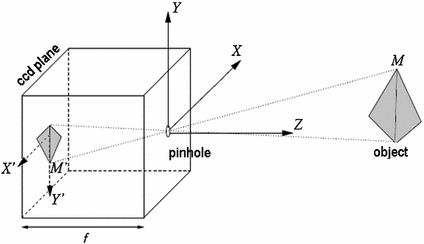
The negative sign is generally changed by considering the image projected between the viewing point and the object (Fig. 1).

In the pinhole assumption, the complex dioptric lens system is substituted by an ideal single lens, infinitesimally thin, thus the optical system agrees with the following assumptions [15]:

all parallel light rays are concentrated on the focus;
no refraction is induced to all rays passing through the lens center;
all non-centered rays are deviated in correspondence of the middle plane.

Other assumed hypotheses, adopted when dealing with digital images are:

the optical axis is perfectly orthogonal to the sensor plane and centered on it;
the sensor gauge is organized by a two perfectly orthogonal cell disposition.

Fig. 1

Scheme of pinhole camera view

2.1 Identification of Grid Images

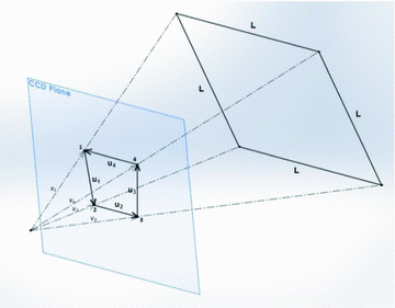
In this section we assume that the image is simply constituted by a regular square grid. In the next section the association of a grid to a general image is discussed. Figure 2 shows the projection of a simple square on the CCD plane that is reversed, as usually. The geometry projected on the plane is given by the four vectors connecting the observation point to the square corners.

Once the image is digitally acquired, each vector v associated to a point is known in its direction, while its magnitude remains unknown. All unknowns are represented by the moduli associated to the respective vectors. According to this logic, all vectors U are computed as differences of vectors V (Fig. 2). In the following, the vectors V will be addressed making use of respective unit vectors: $\mathbf{V} = \mathrm{m} \cdot \mathbf{v}$ .

Fig. 2

Vectors identifying the positioning of element nodes

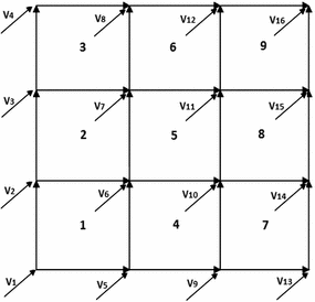
Fig. 3

Nomenclature of a $3\times 3$ grid

Making reference to the $3\times 3$ grid represented in Fig. 3, the first element gives the following equations:

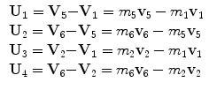
$\begin{aligned} \begin{array}{l} \mathbf{U}_\mathbf{1} =\mathbf{V}_\mathbf{5} \mathbf{-V}_\mathbf{1} =m_5 \mathbf{v}_5 -m_1 \mathbf{v}_1 \\ \mathbf{U}_2 =\mathbf{V}_6 \mathbf{-V}_5 =m_6 \mathbf{v}_6 -m_5 \mathbf{v}_5 \\ \mathbf{U}_3 =\mathbf{V}_2 \mathbf{-V}_\mathbf{1} =m_2 \mathbf{v}_2 -m_1 \mathbf{v}_1 \\ \mathbf{U}_4 =\mathbf{V}_6 \mathbf{-V}_2 =m_6 \mathbf{v}_6 -m_2 \mathbf{v}_2 \\ \end{array} \end{aligned}$

(2)

Being the grid formed by equal squares, several conditions can be imposed to each of them – note that not all of them are independent – represented in Table 1.

Table 1

Vector and scalar conditions for a square grid

Geom. condition	Vector eq.	Number of scalar eqs
$U_2\,\Vert \,U_3$	$U_2 \times U_3 = 0$	3
$U_1\,\Vert \,U_4$	$U_1 \times U_4 = 0$	3
$U_1 \perp U_2$	$U_1 \cdot U_2 = 0$	1
$U_2 \perp U_4$	$U_2 \cdot U_4 = 0$	1
$U_3 \perp U_4$	$U_3 \cdot U_4 = 0$	1
$U_1 \perp U_3$	$U_1 \cdot U_3 = 0$	1
	$U_1 \cdot U_1 = L^2$	1
	$U_2 \cdot U_2 = L^2$	1
	$U_3 \cdot U_3 = L^2$	1
	$U_4 \cdot U_4 = L^2$	1

The equations given in the previous Table 1 generates, using the modules as the unknowns, the following 14 equations (first two are vector equations):

$\begin{aligned} \begin{array}{l} m_1 m_5 \left( {\mathbf{v}_5 \times \mathbf{v}_1 } \right) -m_1 m_6 \left( {\mathbf{v}_6 \times \mathbf{v}_1 } \right) -m_2 m_5 \left( {\mathbf{v}_5 \times \mathbf{v}_2 } \right) -m_2 m_6 \left( {\mathbf{v}_6 \times \mathbf{v}_2 } \right) =\mathbf{0} \\ m_1 m_2 \left( {\mathbf{v}_1 \times \mathbf{v}_2 } \right) -m_1 m_6 \left( {\mathbf{v}_1 \times \mathbf{v}_6 } \right) -m_2 m_5 \left( {\mathbf{v}_5 \times \mathbf{v}_2 } \right) +m_5 m_6 \left( {\mathbf{v}_5 \times \mathbf{v}_6 } \right) =\mathbf{0} \\ \end{array} \end{aligned}$

(3)

$\begin{aligned} \begin{array}{l} m_1 m_5 \left( {\mathbf{v}_1 \cdot \mathbf{v}_2 } \right) -m_1 m_6 \left( {\mathbf{v}_1 \cdot \mathbf{v}_6 } \right) -m_5 m_5 \left( {\mathbf{v}_5 \cdot \mathbf{v}_5 } \right) +m_5 m_6 \left( {\mathbf{v}_5 \cdot \mathbf{v}_6 } \right) =0 \\ -m_2 m_6 \left( {\mathbf{v}_2 \cdot \mathbf{v}_6 } \right) +m_2 m_5 \left( {\mathbf{v}_2 \cdot \mathbf{v}_5 } \right) -m_5 m_6 \left( {\mathbf{v}_5 \cdot \mathbf{v}_6 } \right) +m_6 m_6 \left( {\mathbf{v}_6 \cdot \mathbf{v}_6 } \right) =0 \\ m_1 m_2 \left( {\mathbf{v}_1 \cdot \mathbf{v}_2 } \right) -m_1 m_6 \left( {\mathbf{v}_1 \cdot \mathbf{v}_6 } \right) -m_2 m_2 \left( {\mathbf{v}_2 \cdot \mathbf{v}_2 } \right) +m_2 m_6 \left( {\mathbf{v}_2 \cdot \mathbf{v}_6 } \right) =0 \\ m_1 m_1 \left( {\mathbf{v}_1 \cdot \mathbf{v}_1 } \right) -m_1 m_2 \left( {\mathbf{v}_1 \cdot \mathbf{v}_2 } \right) -m_1 m_5 \left( {\mathbf{v}_1 \cdot \mathbf{v}_5 } \right) +m_2 m_5 \left( {\mathbf{v}_2 \cdot \mathbf{v}_5 } \right) =0 \\ \end{array} \end{aligned}$

(4)

$\begin{aligned} \begin{array}{l} m_1^2 \sum \limits _{i=1}^3 {\nu _{1\left( i \right) }^2 } -2m_1 m_3 \sum \limits _{i=1}^3 {\left( {\nu _{1(i)} \nu _{5(i)} } \right) ^{2}+m_5^2 \sum \limits _{i=1}^3 {\nu _{5\left( i \right) }^2 } } =L^{2} \\ m_5^2 \sum \limits _{i=1}^3 {\nu _{5\left( i \right) }^2 } -2m_5 m_6 \sum \limits _{i=1}^3 {\left( {\nu _{5(i)} \nu _{6(i)} } \right) ^{2}+m_6^2 \sum \limits _{i=1}^3 {\nu _{6\left( i \right) }^2 } } =L^{2} \\ m_2^2 \sum \limits _{i=1}^3 {\nu _{2\left( i \right) }^2 } -2m_2 m_1 \sum \limits _{i=1}^3 {\left( {\nu _{2(i)} \nu _{1(i)} } \right) ^{2}+m_1^2 \sum \limits _{i=1}^3 {\nu _{1\left( i \right) }^2 } } =L^{2} \\ m_6^2 \sum \limits _{i=1}^3 {\nu _{6\left( i \right) }^2 } -2m_6 m_2 \sum \limits _{i=1}^3 {\left( {\nu _{6(i)} \nu _{2(i)} } \right) ^{2}+m_2^2 \sum \limits _{i=1}^3 {\nu _{2\left( i \right) }^2 } } =L^{2} \\ \end{array} \end{aligned}$

(5)

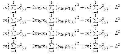
All above equations give a non-linear (quadratic) system of equations where the unknowns are vector magnitudes. If one considers all possible combinations of products of unknowns as unknowns themselves, they turn to be 10 for a single element, with 14 equations each. As an example, for the element n. 1 of Fig. 3, the 10 unknowns are listed in Table 2.

Table 2

List of unknowns produced by a single element

Unknowns
1		6
2		7
3		8
4		9
5		10

The full system of equations is therefore over-determined and the solution can be found solving all the quadratic unknowns involved. After the full solution, each vector magnitude is computed by the root square of the quadratic unknowns. Furthermore, the mixed product of the unknowns can be used to check the accuracy of the solution gained.

2.2 Virtual Image Embedded on a Picture

If an image is present on a surface, this can be associated to a virtual grid. The point is to guarantee that the grid follows the changes of the image, due to movements of the surface that can be considered as a combination of rigid and deformable displacements.

This can be accomplished by considering the grid as a mesh of bilinear finite elements, whose movements guarantee the continuity of the surface. Each element contains a part of the initially flat image; this information is maintained in a natural coordinate system as shown in Fig. 4.

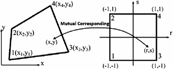
Fig. 4

Physical/Natural coordinate systems

Such reference approach is particularly suitable to compare elements that are initially irregular or become irregular due to large displacements on the image. Therefore, each sub-image is interpolated though a cubic spline approach. By this procedure, each element is always square-represented and keeps the same image content. In Fig. 5 is shown an example of how interpolation deforms the image.

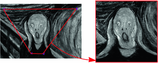
Fig. 5

Change from physical to natural coordinates

2.3 Results on Out of Plane Deformation

The data here presented, apart the very next subsection, refers to all effective pictures taken with a focal distance equal to 29 mm, corresponding to a printed paper positioned at 1500 mm from the ideal lens center. All images have been obtained with an aperture equal to 1/8 to increase overall focus depth.

2.3.1 Test of the Procedure on Exact Grids

The theoretical correctness of the procedure presented has first of all been investigated through the application on a simulated grid (no pictures does effectively exist) that has been deformed applying one or two finite curvatures. We can see that the reconstruction is perfectly accurate (no digital error on pixel definitions is present since pixel positions are recorded with 12 digit precision) only if the local orientation of the grid causes a single curvature change $(R_{c} = 1430\,\mathrm {mm})$ . It is interesting to highlight that the application of a small noise (1 % of the diagonal length of a single element) reduces considerably the precision if the results are very accurate, but does not appreciably changes the behavior if discrepancies are already encountered when data are not affected by noise.

From the above reasons, it is clear that the assumption of square grid to maintain its shape is very strong, difficult to obtain when double curvature are present. This means that the size of the elements of the grid should be taken as small as the curvature increases. As a matter of fact, the last row in Table 3 shows much better results in this case, as expected (double curvature keeping the same equivalent value than single curvature case).

Table 3

Noise effect on accuracy for various curvatures

	No noise (%)	Added noise (%)
Plane grid	$\sim$ 1e-10	4.06
Single curvature	$\sim$ 1e-10	4.87
Double curvature	23.13	24.21
D.curv. refined el.	13.61	15.93

2.3.2 Tests on Pictures of Printed Grids

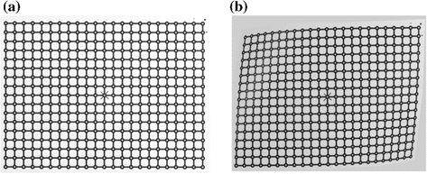
The grid is printed on a sheet of paper that is first photographed in a plane orthogonal to the focal axis, and the second picture considers the sheet deformed in various ways, such as the one shown in Fig. 6.

Four cases are here presented; (i) it concerns a $5-10-15^{\circ }$ rigid rotation of the paper on a vertical axis as to generate a prospective view; (ii) it regards a simple half-fold oriented as the vertical axis in the center, and folded at a corner; (iii) the paper leaned on a cylinder (diameter = 450 mm) with a vertical axis; (iv) the paper applied on the same cylinder with the sheet base inclined of $30^{\circ }$ .