Cortical Surface Representation Using Currents. The concept of representing a surface as a current derives from Faraday’s law of induction in physics, which states that the variation of any magnetic vector field W through a surface S induces a current in the space within a wire loop delimiting S [10]. The intensity of the current is proportional to the variation of the flux of this magnetic field, which mathematically translates as an integration of the vector field elements along the shape unit normal vectors n: , where denotes Lebesgue measure on the surface. Hence, a surface can be geometrically defined as the collection of local fluxes for all possible vector fields traversing it. In this regard, W is defined as a Reproducing Kernel of Hilbert Space (RKHS) spanned by convolutions between a square integrable vector field and a Gaussian smooth kernel . The rate of decay of the kernel denotes the scale under which the geometric details of the surface –when converted into a current– are overlooked.

A vector can be measured at a location x for any fixed points y and vectors as a convolution between the kernel and vectors : , where the couple is called a momentum. On the other hand, the space of currents is defined as a vector space containing the set of all continuous linear maps from W to (i.e. the dual space of W). Any current in is then defined as: , where defines a Dirac delta current. 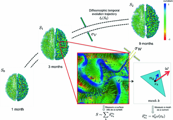Although it is scale-dependent, W enables to densely ‘convert’ the surface S into a current by locally measuring these localized Dirac delta currents and summing them up: ; thus S becomes fully parameterized by its meshes (triangles) k and normals located at each center of these meshes and approximated using the Dirac delta currents located at the center of each of its meshes k (Fig. 1). Hence, any surface can be decomposed into an infinite sum of Dirac delta currents which act as basis vectors in the space of currents . More importantly, the current space is endowed with a metric that enables us to measure the distance between two shapes (i.e. two currents): and , thereby elegantly paving the way to formulate and solve geodesic surface matching problems.

Spatiotemporal Diffeomorphic Current-based Surface Regression Model. Considering a set of longitudinal cortical surfaces acquired at different timepoints , we estimate a spatiotemporal surface growth model that successively deforms the baseline shape onto the consecutive shapes: . This deformation process is guided by the diffeomorphic mapping , which identifies for each mesh the optimal evolution trajectory as a solution of the following flow equation:
Here denotes the time-dependent deformation velocity. To guarantee the smoothness and the invertibility of the estimated deformation trajectory , the velocity field V is defined as a RKHS with a Gaussian kernel . The deformation kernel decays at a rate denoting the scale under which deformations are locally similar to the identity map (no deformation). The time-dependent velocity writes as , with M the number of meshes in the baseline shape [10]. For a static shape , the vector field W associated with it is closely spanned by the momenta (x, n). To cause to become dynamic and warp it onto different shapes, an external momentum of the deformation field locally acts on its Dirac delta currents to geodesically deform it into the consecutive observed shapes. The estimation of the momenta fully defines the surface deformation process from to . This is achieved through conjugate gradient descent algorithm minimizing the following energy:

Where denotes a trade-off parameter between the total kinetic energy of the deformation (first term) and the similarity measure between the deformed baseline shape and the consecutive ground truth observations (second term).

Current-Based Geometric and Dynamic Features Learning. In the training stage, we estimate a cortical surface growth scenario for each infant in our training dataset using the available MR acquisition timepoints. We first register all the baseline surfaces of the training subjects into a common space. Then, for each warped baseline shape in this space, we estimate its temporal evolution trajectory. Both of these steps are achieved using the current-based deformation model, thereby providing a normalized current space, where all subjects’ longitudinal shapes become ‘linked’ in space and time. This facilitates inter-subject comparison of deformation features estimated at any timpoint falling in the in-between obervations interval . At this point, we introduce the notion of a cloud , which is composed of points with x a vertex belonging to any baseline shape in the training data and as its corresponding temporal deformation trajectory. In other words, a point c(x, t) in the cloud locates the new position of any baseline vertex x at a specific timepoint t. Here, the 3D position of any baseline vertex x defines the geometric feature and its evolution trajectory defines the dynamic feature of the learnt model. We will exploit both of these features to predict the evolution trajectory for a new baseline shape.

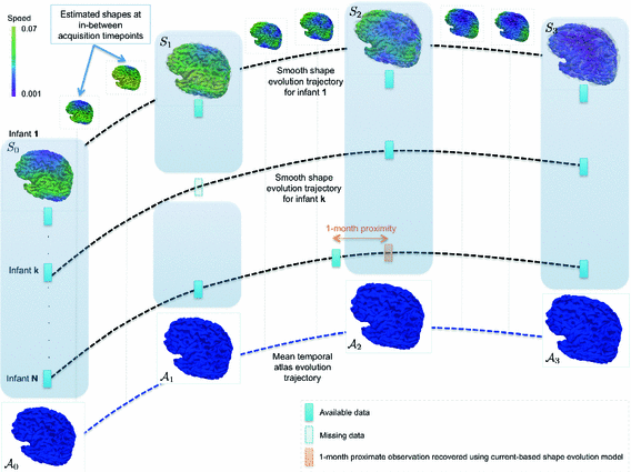
Cortical Spatiotemporal Atlas Estimation. For each of the most commonly shared acquisition timepoints , we build an empirical mean atlas by computing the mean 3D position of the spatiotemporally aligned training subjects. We also include the estimated shapes using the current-based surface growth model for the atlas building if these shapes were acquired at month gap from the ground-truth shape (Fig. 2). Indeed, at month gap, the current-model recovers neighboring information with high accuracy (mean std = ). One could intuitively explain this by recalling the principle of the least action in a classical mechanical Lagrangian framework, which grounds the diffeomorphic geodesic surface deformation framework. This strategy allows us to include more data into building the temporal atlas with and to better capture inter-subject variability.