mm). Two scans of each subject were acquired and stitched together to cover all lumbar IVDs from T12/L1 to L4/L5. The acquisition time was 7 min 50 s per block.
Although all 12 subjects were ‘asymptomatic’ healthy volunteers, disc degeneration was observed in 4 subject (6/60 lumbar IVDs) by a trained radiologist. Such abnormal findings are common in the asymptomatic population and are in accordance with numbers reported in previous clinical studies [5]. Other radiological findings included vertebral haemangiomas in 2 cases and several Schmorl’s nodes (vertebral endplate fracture) of varying dimensions.
All cases were manually segmented and used to generate the statistical shape models and to quantitatively evaluate the segmentation algorithm.
The medical research ethics committee of the University of Queensland approved the current study and written informed consent was obtained from all participants involved.
2.2 Image Pre-processing
Two slightly overlapping serial blocks were acquired for each subject in this study and stitched together using a customised algorithm explained in more details in [12]. The pre-processing steps further included an intensity inhomogeneity correction based on the N4 bias field correction algorithm [16], smoothing by gradient anisotropic diffusion (15 iterations with time step 0.01 and conductivity 0.25) and signal intensity value standardisation by atlas matching of the image histograms extracted from the spinal column.
2.3 Image Segmentation
The segmentation algorithm is based on the method of active shape models (ASM) [2]. The ASM is initialised by a series of object recognition techniques as presented in [12]. This method estimates the spine curve and detects centres of vertebral bodies. The initial IVD models are placed half way between detected vertebral bodies and oriented to follow the estimated spine curve. The algorithm was successful in detecting 58/60 vertebral bodies. In 2 cases, the lower-most vertebral body L5 was missed and annotated manually.
This section outlines the traditional and the multi-level statistical shape models, presents the segmentation scheme and parameters, and explains the validation procedure.
2.3.1 Traditional Statistical Shape Models
After initial shape alignment (the generalised Procrustes alignment [6]), a point distribution can be defined for the positions of spatially corresponding shape vertices  for
for  shapes consisting of
  vertices. The mean shape
  and covariance matrix
  are computed. Each shape
  is represented as an
  -dimensional vector
  . The shape vectors can be represented in the form of:
 where
where  are the eigenvectors of the covariance matrix
  (with corresponding eigenvalues
  ) and
) and  are the weights of each mode of variation (also called shape parameters) parameterising the shape
  . The number of used modes of variation is usually reduced since a smaller number of modes
  can explain most variation in the dataset.
 for
for  shapes consisting of
  vertices. The mean shape
  and covariance matrix
  are computed. Each shape
  is represented as an
  -dimensional vector
  . The shape vectors can be represented in the form of:
 are the eigenvectors of the covariance matrix
  (with corresponding eigenvalues
  ) and
) and  are the weights of each mode of variation (also called shape parameters) parameterising the shape
  . The number of used modes of variation is usually reduced since a smaller number of modes
  can explain most variation in the dataset.
One statistical shape model from all lumbar discs was generated. The point correspondences were obtained using SPHARM parameterisation and groupwise optimisation of the description length [4].
2.3.2 Multi-level Statistical Shape Model
The MSSM presented by Lecron et al. [7] applies principles of multi-level component analysis [15] to describe variations in hierarchical structures. In the example of the lumbar spine in this study, the structure of  intervertebral discs is divided into
  groups of disc levels (T12/L1 to L4/L5) where each groups consists of 12 discs of the same level of different subjects. The multi-level component analysis finds independent components of within-class and between-class variation from a decomposition of each shape belonging to a group
  as:
as:
 where
where  is the mean shape of class
  . This decomposition defines two-level hierarchical model where the within-class variation (same IVD level) and between-class variation are modelled independently.
 intervertebral discs is divided into
  groups of disc levels (T12/L1 to L4/L5) where each groups consists of 12 discs of the same level of different subjects. The multi-level component analysis finds independent components of within-class and between-class variation from a decomposition of each shape belonging to a group
  as:
as:
 is the mean shape of class
  . This decomposition defines two-level hierarchical model where the within-class variation (same IVD level) and between-class variation are modelled independently.
A lumbar spine  can be reconstructed from the components of within-class variation
  and the between-class variation
  :
:
 where
where  and
and  ,
,  are respectively the within-class and between-class shape parameters for the spine
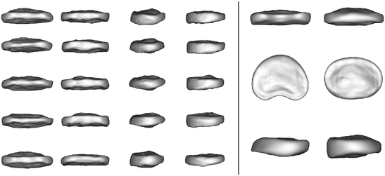
  . The within-class component describes global anatomical differences between individual subjects, whereas the between-class component describes changes between IVDs at different levels of the lumbar spine (from T12/L1 to L4/L5). As such, both components are important for a successful segmentation. The most important modes of variation are presented in Fig. 1.
 can be reconstructed from the components of within-class variation
  and the between-class variation
  :
:
 and
and  ,
,  are respectively the within-class and between-class shape parameters for the spine
  . The within-class component describes global anatomical differences between individual subjects, whereas the between-class component describes changes between IVDs at different levels of the lumbar spine (from T12/L1 to L4/L5). As such, both components are important for a successful segmentation. The most important modes of variation are presented in Fig. 1.
Fig. 1
Modes of variation of the multi-level statistical model. First mode of the within-class component is shown in the left panel (posterior and lateral views). The mode primarily captures a relative IVD narrowing (inferior–superior). The first mode of the between-class component is shown in the right panel (posterior, superior and lateral views). The mode describes anterior–posterior wedging and changes from a circular to a ‘bean’ like shape. These are typical differences between inferior and superior lumbar IVDs

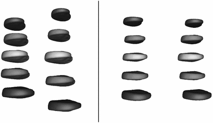
Fig. 2
General model of coarse variation of the lumbar spine. The first mode (left) describes the extension of the lumbar spine and some relative changes in the IVD size. The second mode (right) describes primarily the extent of the lordosis. For visualisation purposes, the statistical mean shape was inserted to the locations described by the coarse model and scaled accordingly
In contrast to Lecron et al. [7], all shapes are initially aligned (the generalised Procrustes alignment [6]) and the MSSM do not contain any information on relative poses of the IVDs, allowing to model uniquely the variation in shape. We model the coarse global variation in relative disc positions and their scale by a simplified statistical model. A  matrix containing the centroid points of each IVD and its scale (in each row) is constructed for every lumbar spine and the principle component analysis is performed. This analysis is used as a rough control over the global shape of the segmented spine and allows the MSSM to focus on changes between individual shapes. The first two modes of the global lumbar spine variation are shown in Fig. 2.
 matrix containing the centroid points of each IVD and its scale (in each row) is constructed for every lumbar spine and the principle component analysis is performed. This analysis is used as a rough control over the global shape of the segmented spine and allows the MSSM to focus on changes between individual shapes. The first two modes of the global lumbar spine variation are shown in Fig. 2.
2.3.3 Shape Deformation
The shape deformation procedure is an iterative process driven by grey level profile matching. Initially, training profiles are extracted from the manually segmented shapes in the database. At each iteration, grey level profiles  of lengths
 ![$$2R+1 > 2L+1$$” src=”/wp-content/uploads/2016/03/A323246_1_En_15_Chapter_IEq30.gif”></SPAN></p>
<div class='tao-gold-member'>
<div>Only gold members can continue reading. <a href='/login'>Log In</a> or <a href='/register'>Register</a> to continue</div>
</div>
<p></p>
<div class=]()
 of lengths
 Stay updated, free articles. Join our Telegram channel

Full access? Get Clinical Tree


