of Lumbar Vertebrae Slices from CT Images

. The energy function of the CRF defines a posterior probability distribution $P(\mathbf {x} \mid \mathbf {y})$ for a set of class labels $\mathbf {x}$ for the superpixels, given a set of features $\mathbf {y}$ describing the superpixels. The energy function can be written as a sum of first- and second-order potential functions in the form

$\begin{aligned} \begin{aligned} E(\mathbf {x}, \mathbf {y}) = \sum _{i \in \mathcal {S}} \underbrace{\psi (\mathbf {y}_i \mid x_i)}_{\text {Data term}} + \lambda \sum _{i \in \mathcal {S}} \sum _{j \in \mathcal {N}_i} \underbrace{\phi (\mathbf {y}_i, \mathbf {y}_j \mid x_i, x_j)}_{\text {Smoothness term}} \end{aligned} \end{aligned}$

(1)

where $\mathcal {N}_i$ is the set of neighbours of superpixel

. The constant $\lambda$ controls the relative importance of the data and smoothness terms. The CRF formulation enables maximum a posteriori (MAP) inference of the labels $\mathbf {x}$ to be carried out efficiently using graph cuts. We use the min-cut/max-flow algorithm of [4] to find the optimal solution.

We define the potential functions of (1) by using supervised learning on labelled superpixel features and deriving constraints using the resulting trained models. Sections 3 and 4 describe the superpixel features used to learn the constraints and how they are incorporated into the CRF potential functions.

3 Superpixels

We use the Simple Linear Iterative Clustering (SLIC) [1, 16] algorithm to partition the image into superpixels. As shown in Fig. 1, boundaries of superpixels tend to coincide with boundaries of anatomical objects, enabling an accurate pixel-level segmentation to be recovered from the classified superpixels. The primary advantages of using superpixels are twofold: firstly, as the number of nodes in the graph decreases significantly from a pixel-level graph, there is a corresponding reduction in computational complexity. Secondly, multiple features can be extracted from the superpixel regions which can help to discriminate between the classes more effectively.

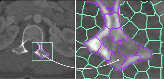
Fig. 1

The left figure shows a CT slice with ground truth contour (magenta) for a section of the vertebra. The right figure shows boundaries for superpixels assigned to the vertebra class (magenta) and background class (cyan). The superpixels preserve the boundary detail of the vertebrae (color figure online)

We aim to characterise the superpixels by extracting multiple features from them that incorporate information about intensity, texture, location and edge response. As described in the next section, these features are used to discriminate between the vertebra and background superpixels by learning a classifier and distance metric on a set of ground truth images. We emphasise that this training occurs only once, after which the trained models can be used in the CRF potential functions for any further images.

The superpixel features are summarised in Table 1. The feature vector for a superpixel

is a concatenation of the individual features:

Table 1

Superpixel features ( $$p_n$$

denotes the $$n$$

th percentile)

Feature	Description	Dimension
$\mathbf {y}_i^{T_1}$	Concatenation of intensity histogram from superpixel and average histogram from neighbours $\mathcal {N}_i$	20
$\mathbf {y}_i^{T_2}$	SIFT descriptor calculated at the centroid of superpixel	128
$\mathbf {y}_i^{L_1}$	Mean, $p_{10}$ and $p_{90}$ of the row and column pixel coordinates in the superpixel, centred on the matched contour region	6
$\mathbf {y}_i^{L_2}$	Mean, $p_{10}$ and $p_{90}$ of the matched contour distance transform gradient in the superpixel, in both the horizontal and vertical direction	6
$\mathbf {y}_i^{E_1}$	Mean, $p_{10}$ and $p_{90}$ of the LoG response within the superpixel, taken over 4 scales	12
$\mathbf {y}_i^{E_2}$	Mean, $p_{10}$ and $p_{90}$ of the structure tensor eigenvalues of the superpixel, taken over 4 scales	24

$\begin{aligned} \begin{aligned} \mathbf {y}_i = [\mathbf {y}_i^T, \mathbf {y}_i^L, \mathbf {y}_i^E]^{\top }. \end{aligned} \end{aligned}$

(2)

We exhaustively tested different subsets of the features, but found that the best performance was obtained by combining all features. The features were chosen in part for their generality and as a consequence are directly applicable to different imaging modalities such as MRI [9].

The first set of features $\mathbf {y}_i^T$ characterise the intensity and textural properties of the superpixels. They take the form of normalised intensity histograms over the pixels within each superpixel and SIFT [14, 16] descriptors of a fixed size calculated at the superpixel centroids.

The location features are based on a local coordinate system for each vertebra. This helps segmentation by providing features that describe the superpixel’s relative location. The local coordinates are obtained by matching a contour to the top of the vertebral body. We do this by first (automatically) cropping the ground truth segmentation contours above their centroids, so that the resulting contour set $\mathcal {C}$ corresponds to the upper, roughly semi-circular, boundary of each vertebral body in the ground truth set. Each ground truth image is therefore associated with a single contour $C \in \mathcal {C}$ and our goal is to find the best matching contour of the set for a new image. We use a Laplacian of Gaussian (LoG) filter to detect the outer boundary of the vertebra and search over the image to find the point where the average LoG response along the contour is greatest. The best match is the contour with the maximum response of the set. Features are derived from the matched contour region by centring the pixel coordinates at the region’s centroid and computing the gradient of the distance transform [9]. While the matching process depends on the presence of an adequate number of ground truth contours, in practice only an approximate match to the vertebra is required to derive the location features. Using a set of generated synthetic contours is a possibility in cases where the ground truth data is very limited.

Finally, the features in $\mathbf {y}_i^E$ are distinctive of superpixels at the edges and corners of the vertebrae and help to separate the vertebra and background classes around the boundary. We take the LoG response within the superpixel over 4 different scales to form the first feature vector. The second feature vector is formed from the eigenvalues of the structure tensor [12] within the superpixel, taken over 4 scales.

4 Potential Functions

We next describe the potential functions used in (1). Both the data and smoothness terms of the CRF are based on the characteristics learned from superpixel training examples.

We first convert the pixel-level ground truth labels into superpixel-level labels by assigning each superpixel to the class with the majority vote; as Fig. 1 illustrates, there is little ambiguity in this assignment. We then use the superpixel feature/label examples to train a support vector machine (SVM) [5] using an RBF kernel, given by

$\begin{aligned} \begin{aligned} K(\mathbf {y}_i, \mathbf {y}_j) = \exp {\left( -\gamma ||\mathbf {y}_i - \mathbf {y}_j||_2^2 \right) } \end{aligned} \end{aligned}$