1 cm in diameter. Our ultimate goal is to create a robust system for early detection and classification, as well as tracking, of small-size nodules before they turn into cancerous. The entire development in the chapter is model-based and data-driven, allowing design, calibration and testing for the CAD system, based on archived data as well as data accrued from new patients. We provide standard development using two clinical datasets that are already available from the ELCAP and LIDC studies.
1 Introduction
In this chapter, we highlight a state-of-the-art analytic approach to lung nodule analysis using low dose CT (LDCT) of the human chest. Our focus is on small-size nodules ( 1 cm in diameter) that appear randomly in the lung tissue. Radiologists diagnose these nodules by visible inspection of the LDCT scan. Despite the wide range of nodule classifications among radiologists, the nodule classification of Kostis et al. [1] is found to be particularly useful in the algorithmic evaluation presented in this work. Nodules in Kostis’s work are grouped into four categories:(i) well-circumscribed where the nodule is located centrally in the lung without being connected to vasculature; (ii) vascularized where the nodule has significant connection(s) to the neighboring vessels while located centrally in the lung; (iii) pleural tail where the nodule is near the pleural surface, connected by a thin structure; and (iv) juxta-pleural where a significant portion of the nodule is connected to the pleural surface.
1 cm in diameter) that appear randomly in the lung tissue. Radiologists diagnose these nodules by visible inspection of the LDCT scan. Despite the wide range of nodule classifications among radiologists, the nodule classification of Kostis et al. [1] is found to be particularly useful in the algorithmic evaluation presented in this work. Nodules in Kostis’s work are grouped into four categories:(i) well-circumscribed where the nodule is located centrally in the lung without being connected to vasculature; (ii) vascularized where the nodule has significant connection(s) to the neighboring vessels while located centrally in the lung; (iii) pleural tail where the nodule is near the pleural surface, connected by a thin structure; and (iv) juxta-pleural where a significant portion of the nodule is connected to the pleural surface.Figure 1 shows examples of small size nodules ( 1 cm in diameter) from the four categories. The upper and lower rows show zoomed images of these nodules. Notice the ambiguities associated with shape definition, location in the lung tissues, and lack of crisp discriminatory features.
1 cm in diameter) from the four categories. The upper and lower rows show zoomed images of these nodules. Notice the ambiguities associated with shape definition, location in the lung tissues, and lack of crisp discriminatory features.Modeling aims at representing the objects with mathematical formulation that captures their characteristics such as shape, texture and other salient features. The histogram of the object’s image provides some information about its texture—the modes of the histogram indicate the complexity of the texture of the object. Figure 2 shows sample of nodules and their histograms. These histograms are essentially bi-modal, for the nodule and background regions, and may be sharpened if the region of interest (ROI) is limited to be around the spatial support of the nodules.
Another difficulty of small-size nodules lies with inabilities of exact boundary definition. For example, radiologists may differ in outlining the lung nodules spatial support as shown in Fig. 3. Difference in manual annotation is common of small objects that have not well-defined description. This adds another dimension of difficulty for automatic approaches, as they are supposed to provide outputs that mimic human experts. In other words, human experts differ among themselves, how would they judge a computer output? Validation of automatic approaches for lung nodule detection, segmentation and classification – using only the visible information in an image – is an order of magnitude more difficult than that of automatic face recognition, for example.
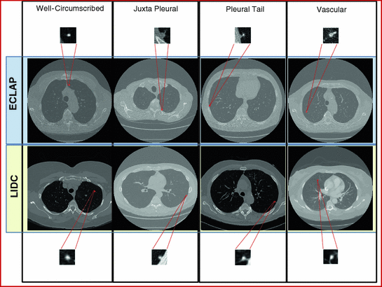
Fig. 1
Examples of lung nodules of size below 10 mm from two clinical studies. The upper and lower rows show zoomed pictures of the nodules
Farag [2] studied the behavior of the intensity versus the radial distance of the nodule centroids [2]. The intensity versus radial distance distribution for small nodules was shown to decay almost exponentially. An empirical measure of the region of support of the nodules was derived based on this distribution. This approach has been tested further on three additional clinical studies in this work and has shown to hold true. The summation of the intensities of Hounsfield Units (HU) in concentric circles (or ellipses) beginning from the centroid of the nodule, decays in a nearly exponential manner with the distance from the centroid.
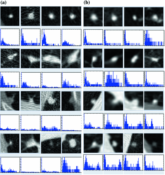
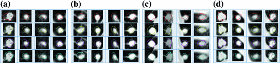
Fig. 2
Sample of nodules and their gray level (Hounsfield Units) histograms. Nodules in left are from ELCAP [3] study and those in the right table from LIDC [4] study. On top row, from left to right: well-circumscribed, vascular, juxta-pleural and pleural-tail nodules, respectively. a Nodules and histograms from the ELCAP study. b Nodules and histograms from the LIDC study
Fig. 3
Manual annotation of the main portion of the spatial support of lung nodules by four radiologists. Note the difference in size and shape of the annotations. a Outlines of fouur well-circumscribed nodules. b Outlines of four vascular nodules. c Outlines of four juxta-pleural nodules d Outlines of four pleural-tail nodules
Figure 4 shows the radial distances for four nodule types from the LIDC clinical studies [4]. This behavior provided a clue for empirically deciding the spatial support (ROI) of the nodules—which is used for auto cropping of the detected nodules. Of course a refinement step is needed to precisely define the exact ROI of the nodule—this is carried out in nodule segmentation. This behavior is similar with the ELCAP study as well.
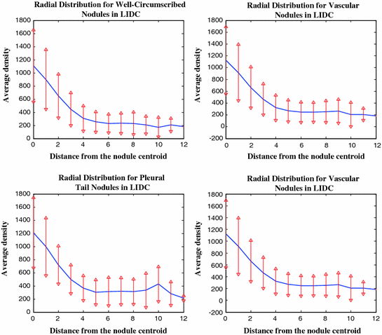
Fig. 4
Distribution of the nodule intensity (HU) for four nodule types manually cropped from the LIDC (over 2000 nodules). For nodules less than 10 mm in diameter, an ROI of size  pixels may be used
pixels may be used Object segmentation is a traditional task in image analysis. Real world objects are hard to model precisely; hence the segmentation process is never an easy task. It is more difficult with the lung nodules due to the size constraints.
Figure 5 shows the average intensity (HU) histograms of the manually cropped nodules in the ELCAP and LIDC screening studies. The histograms are distinctly bimodal and a binary classifier (thresholding) may be used for separating the nodules and non-nodules regions. The decision boundary (threshold) may be selected by various techniques, including fitting one-dimensional Gaussian density for the nodule and non-nodule regions and using the expectation-maximization approach (EM) to estimate the parameters (e.g., [2]). Unfortunately, this approach does not work well due to the uncertainties associated with the physical nodules as previously described.
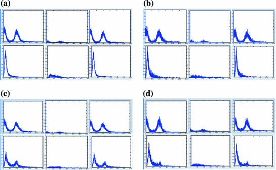
Fig. 5
The intensity (HU) histograms of the manually cropped nodules from the ELCAP and LIDC screening studies. These histograms are bio-modal showing the nodule and non-nodule regions in the ROI. These histograms are used as estimates of the probability density functions in the nodule segmentation process. a Intensity of well-circumscribed nodules for ELCAP (upper) and LIDC (lower) b Intensity of vascular nodules for ELCAP (upper) and LIDC (lower) c Intensity of juxta-pleural nodules for ELCAP (upper) and LIDC (lower) d Intensity of pleural-tail nodules for ELCAP (upper) and LIDC (lower)
There is a vast literature on object modeling and considerably larger literature on the subsequent steps of modeling; e.g., synthesis, enhancements, detection, segmentation, recognition, and categorization. Farag [2] considered a five-step system for modeling of small lung nodules: (i) Acquisition and Enhancement; (ii) Parametric Modeling; (iii) Detection; (iv) Segmentation; and (v) Categorization (Classification) [2]. By constructing a front-end system of image analysis (CAD system) for lung nodule screening, all of these steps must be considered. Activities in the past few years have led to the following discoveries: (1) Feature definitions on small size objects are hard to pin point, and correspondences, among populations, is very tough to obtain automatically; (2) Classical approaches for image segmentation based on statistical maximum a posteriori (MAP) estimation and the variational level sets approaches do not perform well on small size objects due to unspecific object characteristics; (3) Prior information is essential to guide the segmentation and object detection algorithms—the more inclusive the a-priori knowledge, the better the performance of the automated algorithms; (4) An integration of attributes is essential for robust algorithmic performance; in particular shape, texture, and approximate size of desired objects are needed for proper definition of the energy functions outlining the MAP or the level sets approaches. These factors play a major motivational role of this work.
The rest of the material in this chapter will focus on four steps related to an analytic system for lung nodule analysis: lung nodule modeling by active appearance; lung nodule detection; lung nodule segmentation; and lung nodule categorization.
2 Modeling of Lung Nodules by Deformable Models
Deformable models are common in image modeling and analysis. Random objects provide major challenges as shapes and appearances are hard to quantify; hence, formulation of deformable models are much harder to construct and validate. In this work, we devise an approach for annotation, which lends a standard mechanism for building traditional active appearance (AAM), active shape (ASM) and active tensor models (ATM). We illustrate the effectiveness of AAM for nodule detection.
Automatic approaches for image analysis require precise quantification of object attributes such as shape and texture. These concepts have precise definitions, but their descriptors vary so much from one application to another. A shape is defined to be the information attributed to an object that is invariant to scale, origin and orientation [5]. A texture may be defined as the prevalence pattern of the interior of an object [6]. Geometric descriptors identify “features” that are “unique” about an object. Shape, texture and geometric descriptors are major concepts in this work; they will be defined and used in the context of modeling small size objects under uncertainties [7]. The theoretical development in this work falls under the modern approaches of shape and appearance modeling. These models assume the availability of an ensemble of objects annotated by experts—the ensemble includes variations in the imaging conditions and objects attributes to enable building a meaningful statistical database.
Active shape models (ASM) and active appearance models (AAM) have been powerful tools of statistical analysis of objects (e.g., [8, 9]). This section highlights some of the authors’ work on data-driven lung nodule modeling and analysis (e.g., [10, 11]), with focus on active appearance models (AAM).
2.1 Lung Nodule Modeling
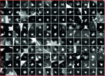
Real world objects may take various forms of details, and may be linear, planar or three-dimensional. In [7], Dryden and Marida, define anatomical landmarks as points assigned by an expert that corresponds between organisms in some biologically meaningful way; mathematical landmarks as points located on an object according to some mathematical or geometrical property, i.e. high curvature or an extremum point; and pseudo-landmarks as constructed points on an object either on the outline or between landmarks. Figure 6 is a sample of small-size nodules smaller than  cm in diameter from the LIDC [4] clinical study, showing the variations that can be captured by shape and appearance models.
cm in diameter from the LIDC [4] clinical study, showing the variations that can be captured by shape and appearance models.Fig. 6
An ensemble of 140 nodules manually cropped from the LIDC study
From a computer vision prospective, AAM and ASM modeling have been used with great successes in objects having distinct landmarks (e.g., [8, 9]). A shape is considered to be a set of  vertices
  ; for the two-dimensional case:
![$$\begin{aligned} {{\varvec{x}}} = \left[ x_{1}; x_{2};\cdots ; x_{n}; y_{1}; y_{2};\cdots ; y_{n}\right] ^{T} \end{aligned}$$](/wp-content/uploads/2016/10/A312883_1_En_8_Chapter_Equ1.gif)
The shape ensemble (realizations of the shape process of a certain object) is to be adjusted (aligned) on the same reference to enable filtering of scale, orientation and translation among the ensemble, per the shape definition. This alignment generates the so-called shape space, which is the set of all possible shapes of the object in question. To align the shapes in an ensemble, various procedures may be used. The Procrustes procedure is common for rigid shape alignments. The alignment process removes the redundancies of scale, translation and rotation using a similarity measure that provides the minimum Procrustes distance.
vertices ; for the two-dimensional case:(1)
Suppose an ensemble of shapes is available with one-to-one point (feature) correspondence is provided. The Procrustes distance between two shapes  and
and  is the sum of squared distance (SSD)
Annotated data of an ensemble of shapes of a certain object carries redundancies due to imprecise definitions of landmarks and due to errors in the annotations. Principal Component Analysis (PCA) may be used for reducing these redundancies. In PCA, the original shape vector is linearly transformed by a mapping such that has  less correlated and highly separable features. The mapping M is derived for an ensemble of N shapes as follows:
are the mean and covariance of X. Therefore, the mean and covariance of z would be:
If the linear transformation M is chosen to be orthogonal; i.e.,  , and selecting it as the eigenvectors of the symmetric matrix
  , this would make
  to be a diagonal matrix of the eigenvalues of
  . The eigenvectors corresponding to the small eigenvalues can be eliminated, which provides the desired reduction. Therefore , x may be expressed as:

where  matrix of
  largest eigen vectors of
  and
and  vector. Equation (5) is the statistical shape model, which is derived using PCA. By varying the elements of b one can vary the synthesized shape x in Eq. (5). The variance of the
  th parameter
  can be shown across the training set to be equal to the eigenvalue
  [8].
[8].
and is the sum of squared distance (SSD)(2)
less correlated and highly separable features. The mapping M is derived for an ensemble of N shapes as follows:(3)
(4a)
(4b)
, and selecting it as the eigenvectors of the symmetric matrix , this would make to be a diagonal matrix of the eigenvalues of . The eigenvectors corresponding to the small eigenvalues can be eliminated, which provides the desired reduction. Therefore , x may be expressed as:(5)
matrix of largest eigen vectors of and vector. Equation (5) is the statistical shape model, which is derived using PCA. By varying the elements of b one can vary the synthesized shape x in Eq. (5). The variance of the th parameter can be shown across the training set to be equal to the eigenvalue [8].2.2 Nodule Annotation
In order to construct the active appearance or active tensor models, we need an annotated ensemble of objects. In case of random objects, the annotation process becomes extremely difficult; it takes yet another level of difficulty with small-size. Yet, the major goal of this work is to address such objects, specifically, small size lung nodules, which are used for early detection screening of possible lung cancer. We used the fuzzy description of lung nodules from Kostis et al. [1] to devise a feature definition approach for four categories of nodules; well-circumscribed, vascularized, juxta-pleural and pleural-tail nodules. Figure 7 illustrates the landmarks that correspond to the clinical definition of these four nodule categories.
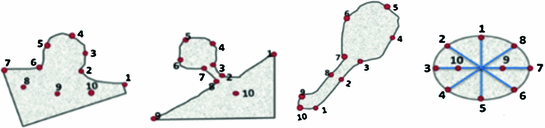
Fig. 7
Definition of Control points (landmarks) for nodules. Right-to- left: juxta-pleural, pleural tail, vascular, a well-circumscribed nodule models
Using the above definitions, we created a manual approach to annotate the nodules. First, we take the experts’ annotation, zoom it and manually register it to a template defining the nodule type/category, and then we select the control points on the actual nodule using the help of the template. This annotation enabled creation of active appearance models, which mimics largely the physical characteristics of lung nodules that cannot be modeled otherwise.
Figure 8 shows examples for the nodule models generated by ensembles from the ELCAP and LIDC clinical lung screening studies. The average nodules (shown in Fig. 8) capture the main features of real nodules. Incorporation of other basis has been studied in Farag et al. [11]. Figure 9 shows examples of AAM nodule models with additional “Eigen nodules”.
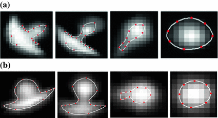
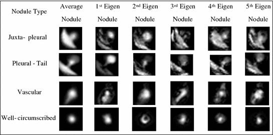
Fig. 8
AAM Models for lung nodules from clinical CT scans. Right-to-left: juxta-pleural, pleural tail, vascular, a well-circumscribed nodule models. a Average nodules from ELCAP study. b Average nodules from LIDC study
Fig. 9
Average and 1st five eigen nodules on ELCAP study
3 Lung Nodule Detection
The above modeling approach has provided tremendous promise in three subsequent steps of lung nodule analysis: detection, segmentation, and categorization. Due to space limitations, we only consider lung nodule detection using the AAM nodule models. Further, we use only a basic detection approach that is based on template matching with normalized cross-correlation (NCC) as similarity measure. Other measures have been examined in our related work (e.g., [11]). We report the detection performance by constructing the ROC of both the ELCAP and LIDC clinical studies. We chose to limit the ensemble size for modeling to be 24 per nodule type for the two studies, to provide a comparison with our earlier work [10]. The ROCs are built to show the overall sensitivity and of the detection process. The textures of the parametric nodules were generated by the analytical formulation in our earlier work (e.g., [10]).
3.1 Clinical Evaluation
ELCAP Data: The ELCAP database [3] contains 397 nodules, 291 identified and categorized nodules are used in the detection process. Results using only the average (mean) template models generated from the AAM approach is examined against parametric nodule models, (i.e. circular and semi-circular) of radius 10, templates in this first set of experiments.
LIDC Data: The Lung Imaging Data Consortium (LIDC) [4] contains 1018 helical thoracic CT scans from 1010 different patients. We used ensembles of 24 nodules per nodule type to design the nodule models (templates) and the rest to test the detection performance.
Figure 10 shows the ROC of 1—specificity versus sensitivity. The results show the superior performance of the AAM-models over the parametric models. In generating these ROC curves, we used the mean in the AAM models as the nodule template (note: in [11] we used other eigen-nodules besides the mean).
We note from Figure 10 that the templates from the ELCAP ensemble provided better performance than those from the LIDC ensemble. This because the wide range of variations in texture information found in the LIDC database, which affects the appearance of the resulting nodule model (template). We used 24 nodules, per nodule type, in both ELCAP and LIDC in order to have even comparison. It is expected that the better AAM models result with larger ensemble size; which is possible with the LIDC study as it contains over 2000 nodules vs. ELCAP which is only few hundreds.
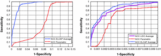
Fig. 10
ROC curves for template matching detection on the ELCAP and LIDC database versus the circular and semi-circular models. a ROC for the ELCAP study. b ROC for the LIDC study
3.2 Extensions
We note that in the ELCAP database, the data acquisition protocol was the same throughout; very low resolution. That was reflected in the AAM model, showing a texture that is relatively more homogenous than that in the LIDC case, which uses data from various imaging centers and various imaging scanners, with somewhat variable range of Hounsfield Units (HU). In general, if we include more nodules in the design, we expect a better appearance modeling; the LIDC database allows such choice.
This section dealt with modeling of small-size lung nodules using two clinical studies, the ELCAP and LIDC. We discussed the process of nodule annotation and the steps to create AAM nodule models. These models resemble the real nodules, thus using them as templates for nodule detection is more logical than the non-realistic parametric models. These types of models add two additional distinctions over the parametric approaches; it can automate the processes of nodule segmentation and categorization. Tensor modeling may also be used to generate the nodule models. From the algorithmic point of view, an adaboost strategy for carrying out the detection may lend speed advantage over the typical cross-correlation implementation used in this work.
4 Nodule Segmentation
This section describes a variational approach for segmentation of small-size lung nodules which may be detected in low dose CT (LDCT) scans. These nodules do not possess distinct shape or appearance characteristics; hence, their segmentation is enormously difficult, especially at small size ( 1 cm). Variational methods hold promise in these scenarios despite the difficulties in estimation of the energy function parameters and the convergence. The proposed method is analytic and has a clear implementation strategy for LDCT scans.
1 cm). Variational methods hold promise in these scenarios despite the difficulties in estimation of the energy function parameters and the convergence. The proposed method is analytic and has a clear implementation strategy for LDCT scans. The lungs are a complex organ which includes several structures, such as vessels, fissures, bronchi or pleura that can be located close to lung nodules. Also, the main “head” of the nodule is what radiologists consider when computing the size. In the case of detached nodules (i.e. well-circumscribed nodules) the whole segmented nodule is considered in size computations and growth analysis, while in detached nodules (i.e. juxta-pleural, vascularized and pleural-tail) the “head” is required to be extracted from the anatomical surrounds. Intensity-based segmentation [13, 14] has been applied to nodule segmentation using local density maximum and thresholding algorithms. These classes of algorithms are primarily effective for solitary nodules (well-circumscribed), however, fail in separating nodules from juxtaposed surrounding structures, such as the pleural wall (i.e., juxta-pleural and pleural-tail nodules) and vessels (vascular nodules), due to their similar intensities.
More sophisticated approaches have been proposed to incorporate nodule-specific geometrical and morphological constraints (e.g., [1, 15–17]). However, juxta-pleural, or wall-attached, nodules still remain a challenge because they can violate geometrical assumptions and appear frequently. Robust segmentation of the juxta-pleural cases can be addressed in two approaches: a) global lung or rib segmentation (e.g., [18]), and b) local non-target removal or avoidance [14]. The first can be effective but also computationally complex and dependent on the accuracy of the whole-lung segmentation. The second is more efficient than the former but more difficult to achieve high performance due to the limited amount of information available for the non-target structures. Other approaches have been proposed in the literature (e.g., [19]), but require excessive user interaction. In addition, some approaches assumed predefined lung walls before segmenting the juxta-pleural nodules (e.g., [20]).
4.1 Variational Approach for Nodule Segmentation
The level set function as a signed distance map is able to capture complicated topological deformations. A level set function 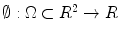 can be defined as the minimum Euclidean distance between the point
  and the shape boundary points. A curve can be initialized inside an object, and then evolves to cover the region guided by image information. The evolving curve within the level set formulation is a propagating front embedded as the zero level of a 3D scalar function
  , where X represents a location in space. In order to formulate the intensity segmentation problem, it is necessary to involve the contour representation. Given an image
 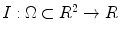 , the segmentation process aims to partition the image into two regions: object (inside the contour denoted by o) and background (outside the contour denoted by b). An error term can be computed by counting the number of correctly classified pixels and then measuring the difference with respect to the total number of pixels. This can be done by summing up the probabilities of the internal pixels to be object and the external pixels probabilities to be classified as background. This is measured by the term:
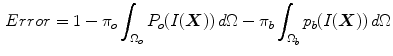
where  and
and  are the probabilities of the object and background according to the intensity values (Gaussian distributions are used to model these regions). Prior probabilities of regions (
 and
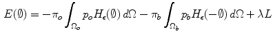
and  ) are involved in the formulation as well. Minimizing this error term is equivalent to minimizing the energy functional:
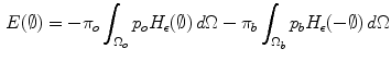
where H is the Heaviside step function and  represents the narrow band region width. An extra term is added to the energy function to represent the contour arc-length (L) which also needs to be minimal to guarantee a smooth evolution. The new energy will be:
where  . The level set function evolves to minimize such a functional using the Euler-Lagrange formulation with the gradient descent optimization:
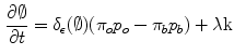
where  is the derivative of the Heaviside function and k is the curvature. Thus, the evolution depends on the local geometric properties (local curvature) of the front and the external parameters related to the input data I. The function
  deforms iteratively according to the above equation, while solving
  gives the position of the 2D front iteratively. Let
  denote the intensity segmented region function representation The Gaussian distribution and prior probabilistic parameters are computed according to the method in [21].
can be defined as the minimum Euclidean distance between the point and the shape boundary points. A curve can be initialized inside an object, and then evolves to cover the region guided by image information. The evolving curve within the level set formulation is a propagating front embedded as the zero level of a 3D scalar function , where X represents a location in space. In order to formulate the intensity segmentation problem, it is necessary to involve the contour representation. Given an image , the segmentation process aims to partition the image into two regions: object (inside the contour denoted by o) and background (outside the contour denoted by b). An error term can be computed by counting the number of correctly classified pixels and then measuring the difference with respect to the total number of pixels. This can be done by summing up the probabilities of the internal pixels to be object and the external pixels probabilities to be classified as background. This is measured by the term:(6)
and are the probabilities of the object and background according to the intensity values (Gaussian distributions are used to model these regions). Prior probabilities of regions ( and ) are involved in the formulation as well. Minimizing this error term is equivalent to minimizing the energy functional:(7)
represents the narrow band region width. An extra term is added to the energy function to represent the contour arc-length (L) which also needs to be minimal to guarantee a smooth evolution. The new energy will be:(8)
. The level set function evolves to minimize such a functional using the Euler-Lagrange formulation with the gradient descent optimization:(9)
is the derivative of the Heaviside function and k is the curvature. Thus, the evolution depends on the local geometric properties (local curvature) of the front and the external parameters related to the input data I. The function deforms iteratively according to the above equation, while solving gives the position of the 2D front iteratively. Let denote the intensity segmented region function representation The Gaussian distribution and prior probabilistic parameters are computed according to the method in [21].4.2 Shape Alignment
This process aims to compute a transformation A that moves a source shape ( ) to its target (
 ). The in-homogeneous scaling matching criteria from [21] is adopted, where the source and target shapes are represented by the signed distance functions
  and
and  respectively. The transformation function is assumed to have scaling components:
 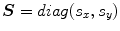 , rotation angle,
  (associated with a rotation matrix R) and translations:
 ![$${{\varvec{T}}} = [T_{x}, T_{y}]^{T}$$](/wp-content/uploads/2016/10/A312883_1_En_8_Chapter_IEq43.gif) A dissimilarity measure to overcome the scale variance issue is formulated by assuming that the signed distance function can be expressed in terms of its projections in the coordinate directions as:
A dissimilarity measure to overcome the scale variance issue is formulated by assuming that the signed distance function can be expressed in terms of its projections in the coordinate directions as: ![$$\mathbf{d}_{\alpha } = [ d_{x}, d_{y}]^{T}$$](/wp-content/uploads/2016/10/A312883_1_En_8_Chapter_IEq44.gif) at any point in the domain of the shape
at any point in the domain of the shape  . Applying a global transformation A on
  results in a change of the distance projections to
  which allows the magnitude to be defined as:
  which implies that
 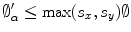 Thus, a dissimilarity measure to compute the difference between the transformed shape and its target representation can be directly formulated as:
) to its target (). The in-homogeneous scaling matching criteria from [21] is adopted, where the source and target shapes are represented by the signed distance functions and respectively. The transformation function is assumed to have scaling components: , rotation angle, (associated with a rotation matrix R) and translations: A dissimilarity measure to overcome the scale variance issue is formulated by assuming that the signed distance function can be expressed in terms of its projections in the coordinate directions as: at any point in the domain of the shape . Applying a global transformation A on results in a change of the distance projections to which allows the magnitude to be defined as: which implies that Thus, a dissimilarity measure to compute the difference between the transformed shape and its target representation can be directly formulated as: