vertebrae (T4-L5) from one normal and one scoliotic magnetic resonance (MR) spine image using six manual and two computerized measurements. Manual measurements were performed by superior and inferior tangents, anterior and posterior tangents, and mid-endplate and mid-wall lines. Computerized measurements were performed by automatically evaluating the symmetry of vertebral anatomy in sagittal cross-sections and volumetric images. The mid-wall lines were the manual measurements with the lowest intra- and inter-observer variability ( and
and  standard deviation, SD). The strongest inter-method agreement was found between the mid-wall lines and posterior tangents (
 SD). Computerized measurements did not yield intra- and inter-observer variability (
 and
and  SD) as low as the mid-wall lines, but were still comparable to the intra- and inter-observer variability of the superior (
 and
and  SD) and inferior (
 and
and  SD) tangents.
1 Introduction
 radiographs of L4/L5 and L5/S1 segments. The manual and computer-assisted measurements proved to be equivalent in terms of variability, the Cobb angle and posterior tangents were the least variable, and the anterior tangents were the most reliable measurements. Street et al. [15] evaluated the reliability of measuring kyphosis manually from different imaging modalities in the case of thoracolumbar fractures. For the Cobb angle measurements, they concluded that plain radiographs were the most reliable measurement modality, followed by computed tomography (CT) and finally by magnetic resonance (MR) imaging.
2 Methodology
2.1 Manual Measurements
 of SVI, measured against reference horizontal or vertical lines that are parallel to the coordinate system of the 3D image.
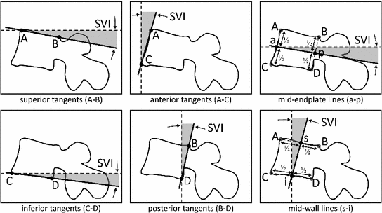
2.2 Computerized Measurements
 of rotation of the local vertebral coordinate system
  (defined by Cartesian unit vectors
  ,
,  and
and  ) around the axes of the global image coordinate system
  (defined by Cartesian unit vectors
  ,
,  and
and  ). Both
  and
and  are right-hand Cartesian coordinate systems, representing left-to-right (
 -axis), anterior-to-posterior (
 -axis) and cranial-to-caudal (
 -axis) direction. The angles
  (i.e. SVI),
  (i.e. coronal vertebral inclination) and
  (i.e. axial vertebral rotation) then represent the rotation of the vertebral coordinate system
  around vectors
  (pitch),
  (roll) and
  (yaw), respectively. If the origin of
  is located at the vertebral centroid and
  is rotationally aligned with the vertebra in
  , anatomically corresponding symmetrical parts of the vertebra can be observed within volumes of interest (VOIs) along positive/negative directions of each axis
  ,
,  . The angles
  of vertebral rotation can be therefore determined by finding the planes of maximal symmetry, which divide the whole vertebra into symmetrical left/right (
 ) halves, and the vertebral body into symmetrical anterior/posterior (
 ) and cranial/caudal (
 ) halves. For each axis
  ,
,  , the symmetrical correspondences of the two halves (
 and
and  ) of a VOI are measured by
  :
:
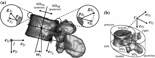
 ), shown for a symmetrical pair of points
  and
and  inside
  . b The vertebral coordinate system
  and the observed volumes of interest (
 encompasses the whole vertebra,
  encompasses the vertebral body)
 is the weighting function, and
  and
and  are the projections of the intensity gradient vectors
  and
and  in the coordinate system
  to the unit vector
  ,
,  , of the coordinate system
  at symmetrical pair of points
  and
and  , respectively, and
  is the number of point pairs inside each VOI (Fig. 2a). By projecting the gradient vectors to
  ,
,  , and by applying the weighting function
  , we retain the gradient components
  and
and  that are relevant for defining the vertebral symmetry in the direction of
  . Two variations of the computerized method were applied for each vertebra. The measurements in 3D automatically evaluated the vertebral rotation in 3D images by maximizing symmetrical correspondences:
 , and the VOI that encompasses the vertebral body is denoted by
  (Fig. 2b). On the other hand, the measurements in 2D automatically evaluated SVI in the same 2D oblique sagittal cross-sections that were used for manual measurements (Fig. 3) by considering only
  that encompasses the vertebral body and reducing its dimensionality to the area of interest (AOI), and maximizing the remaining symmetrical correspondences:
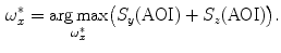
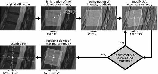
 mm in size to encompass the whole vertebral body of thoracic and lumbar segments. By rotating these planes in 3D, the rotation angles
  are obtained from the inclination of the planes, and the current symmetrical correspondences are evaluated by mirroring the edges of vertebral anatomical structures (obtained from image intensity gradients) over each plane and comparing them to the edges on the opposite side of that plane in an optimization procedure.
3 Experiments and Results
3.1 Images and Observers
 vertebrae between segments T4 and L5 from one normal (
 -year male,
  frontal Cobb angle) and one scoliotic (
 -year male,
  frontal Cobb angle) spine image were included in this study. The T2-weighted MR scans (mean repetition and echo time TR
Related posts:
 Robust Segmentation Framework for Spine Trauma Diagnosis
 Based Tensor Level Set Framework for Vertebral Body Segmentation
Stay updated, free articles. Join our Telegram channel

Full access? Get Clinical Tree


